Universidade Fernando Pessoa
Porto, Portugal
Theoretically, systemic stratigraphy (1) must solve problems that classical stratigraphic approaches, such as lithostratigraphy, biostratigraphy, chronostratigraphy, magnetostratigraphy, etc., could not explained. On the other hand, it must also explain what was already explained by classical approaches1, particularly by the transgressive-regressive facies cycles, which is principal geological concept resulting from classical stratigraphic studies.
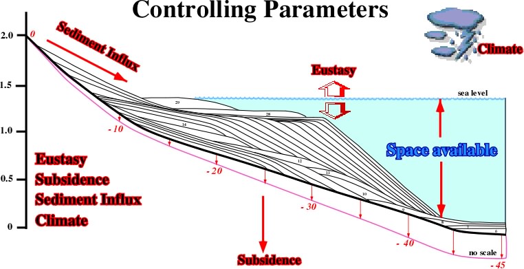
Fig. 8- The main parameters controlling depositional systems are depicted in this no-scale sketch. They are eustasy, subsidence, sediment influx and climate. Landward of the shelf break, the combination of eustasy and subsidence can increase or decrease space for sediment, i.e. shelfal accommodation can be positive or negative. In the first case there is sedimentation, in the second erosion.
The trangressive-regressive cycles represent an assembled picture of lithofacies in relationship to the shoreline location and its position throughout geological time. Suess2 believed that transgression-regression displacements of the shorelines were caused by sea level changes. He used the term eustasy to coin the sea level changes which he believed were global. However, with time, the eustatic concept became unpopular as studies on different continents showed that transgressions - regressions facies cycles did not correlate globally and were mainly due to local uplift and subsidence.
Concerning the sea level changes recorded by geologists, there is always the question of what actually changed:
Was it the elevation of the continent or the absolute level of sea?
“After all”, wrote Macdougal3,
“the sediments only record relative changes, and we know that the continents undergo vertical movements - rocks high in the Alps and the Rockies contain fossils deposited in the ocean, for example, and we know that the oceans were never that deep. However, the case for true sea level change can be made convincingly, if evidence of the sort just described for western North America is found in rocks of the same age from geographically widespread regions. Geologists have mapped the occurrence of various sediment types almost everywhere on earth in considerable detail, and through synthesis of such data there is now a fairly good understanding of the magnitude and timing of global sea level changes. If the rock record indicates that there have been large changes in sea level, the obvious question is, Why?
As far as we know there are really only two possibilities: there must have been changes in either volume of water in the oceans itself, or in the volume of other things that displace the water, such as continents, or islands or ocean ridges. For example, we know that glacial periods are characterized by sea level lowering, because large amounts of the earth's surface water are tied up in ice sheets on the continents. It is estimated that at the height of the last glacial advance, roughly 20.000 years ago, sea level was well over 100 meters lower that it is today. And although much of that ice is gone, there is still a considerable amount of water frozen in the ice caps. If all of it were to melt, sea level would rise by about another 65 meters. That may not sound like much, but a large fraction of the earth's population lives close to sea level, Mexico City would be spared, but much of Los Angeles, New York, Tokyo, and Berlin (to cite just a few examples) would be inundated. Although glacial episodes have major effect on sea level, most of fluctuations that are recorded in Phanerozoic rocks don't occur at times for which there is independent evidence for global ice ages. Most likely they were caused by variations in the volume of the oceanic ridges.”
In order to achieve global or regional correlations, systemic stratigraphy uses physical criteria to define chronostratigraphic intervals and biostratigraphy to determine their age (2). These intervals are considered genetic, in the sense that the rocks inside them are related by facies and bounded by physical surfaces that are, in part, discontinuities. In addition, they are believed to be regional. Some of them are can be even, global. They can be generally mapped within a basin, and sometimes in any basin around the world with a marine base level. Complex interactions between:
(i) Eustasy,
(ii) Tectonics,
(iii) Sediment supply and
(iv) Climate
controls the systemic stratigraphic patterns recognized in the rock record.
Each of these parameters has a stratigraphic signature and a certain rate of change which can be recognized in rock records. P. Vail 5 assumed that: “eustatic changes have an higher rate of change than the other parameters and control the stratal patterns”.
A large majority of the geologists agree that long-term eustatic changes are driven by changes in ocean-basin volume and that these changes are induced by mechanisms of basement movement that act over time periods of tens to hundreds of millions of years and are continental in scope. However, the causes of short-term sea level changes still are very controversial.
The best definition of eustasy is simply “ocean level changes” regardless of causation. It implies vertical (global or local) movements of ocean surface at a particular point, excluding local meteorological, hydrological, and oceanographic changes1.
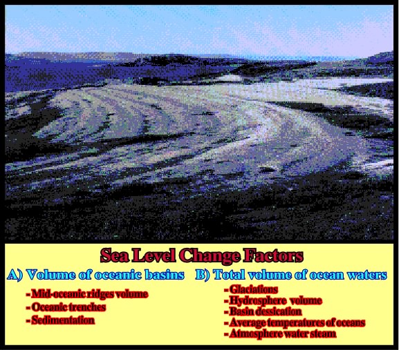
Fig. 9- The back-steps recognized on this photo (Norway) underline successive landward shoreline displacements shoreline induced by relative sea level changes. In this particular example, the relative sea level falls are mainly created by Scandinavia uplift in order to reach isostatic equilibrium.
Three major factors determine the eustatic ocean level changes:
1) Climate changing the ocean water volume,
2) Earth movements changing the ocean basin volume, and
3) Gravitational changes of the ocean level distribution.
The ocean basin volume changes, controlled by earth movements, and ocean water volume changes, mainly controlled by glacio-eustasy (climate), determine the ocean level. However, the ocean level is not equally distributed but rough and uneven due to gravity forming the equipotential surface of the geoid or the geodetic sea level. The vertical ocean level changes may be caused both by real ocean changes, i.e. true eustasy and by geodetic sea level changes (geoidal eustasy). The three ocean variables are:
1) The ocean basin volume, which is a function of vertical and horizontal earth movements (silting up plays a minor role).
2) The ocean water volume, mainly determined by climate and the glacial volume. Juvenile water, water in sediments, water in clouds and lake volumes play a minor role.
3) The ocean level, i.e. the geological eustatic level assumed to be parallel to the Earth's ellipsoid, but via gravity irregularities, changed to the rough and uneven geodetic sea level, or equipotential surface of the geoid.
The eustasy can be illustrated by the variations of level of wine in a cup. The size of the cup simulates the ocean basin volume (fig.10) which can be changed by compressing and expanding the cup (earth movements simulation) causing the rise and fall. The rise and fall of the wine's surface simulates tectono-eustasy. The wine volume in the cup can be changed by drinking and refilling (climate), giving rise to corresponding rises and falls in the wine level (glacial-eustasy).
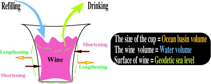
Fig. 10- The ocean basin can be considered as a rubber cup of wine: (i) when you refill it, the wine-level rises, (ii) when you drink it, the wine-level falls, (iii) when you stretch the cup (shortening), the wine-level rises, (iv) if you extend the cup (lengthening), the wine-level falls. In addition, if you take a close look at the surface of the wine you will see that it is not flat, but undulated with highs and lows.
Dilatation depending on the temperature (which is sometimes advocated) plays no significant role. Earth's movements and climate determine the level of the water in the oceans, i.e. the eustatic sea level. In the cup the wine table is not flat but a rough and uneven one (geodetic sea level), i.e. any change in the gravity rise to redistribution in irregularities in the water surface. This metaphor will be better understood if we review the concepts of geoid and eustasy.
The geoid is the equipotential surface of the Earth's gravity field. It is determined by attraction and rotation potentials. The ocean geoid is often termed geodetic sea level2.
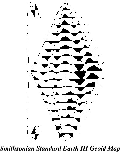
Fig. 11- The sea level profiles show strong irregularities. Sea level is not flat. Large humps and depressions, related with gravity changes and factor control them, are quite evident. Between the high near New Guinea and the low near Maldives, there is a difference of 180 m. In other words, eustatic sea level changes must take into account the local sea level variation induced by gravity anomalies.
The geoid is a function of Earth's gravity field (in turn a function of its structure, density, rheology, and rotation) and of the astronomical gravity, besides the main gravity of the Universe which is thought to be constant. The Earth's density differences and internal flow pattern give rise to the irregular geoid configuration and the magnetic field irregularities.
The sea level profiles of the Smithsonian Standard Earth III geoid map is illustrated in fig. 11. With respect to the Earth's center, one can note that there is a 180 meters sea level difference between the geoid hump at New Guinea and the geoid depression at Maldives Islands. In addition, the present geoid configuration is, of course, not stable. It must have changed with changes in gravity and the factors controlling it. In other words, through geological time the location of humps and depressions of sea level had changed continuously. This feature must be taken into account when proposing stratigraphic global correlations. In fact, this geoid map clearly emphasizes that two areas, not too far apart, can at, at same time, different geological conditions (highstand and lowstand).
As said before, the best definition of eustasy is simply ocean level changes itself instead of crustal tectonic and isostatic movements. Eustasy was also defined as “worldwide simultaneous changes in sea level”, as distinguished from local sea level changes. According to Mörner3 geoid changes must be included under the general term “eustasy” for the following reasons:
1) They have a direct effect on the ocean level changes and most sea level records are faced with the problem of separating the ocean “eustatic” factor from the crustal factor.
2) They affect the ocean level globally (though by different signs) and distinguish from local effects.
3) It will be very hard, almost impossible, to distinguish them from glacial-eustatic and tectonic eustatic changes (3) and will therefore, at any rate, and in the majority of papers, included in term “eustatic changes”.
Five orders of eustatic cycles (fig. 12) have been identified in the geological record. They have been designated as 1st to 5th order cycles1.
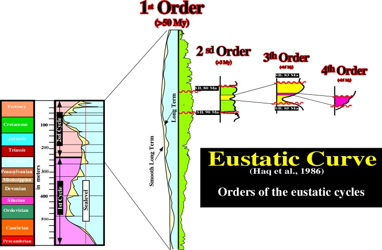
Fig.12- Different orders of eustatic cycles can be recognized on Exxon’s eustatic curve. Since Phanerozoic, there are two 1st order eustatic cycles. The first one defines the Paleozoic and the second one the Ceno-Mesozoic.
The 1st order eustatic cycles correspond to continental flooding cycles defined on the basis of major times of encroachment (landward extension) and restriction of sediments onto the cratons. They are associated with the breakup of supercontinents. They are recognized on all continents and they are believed to be global. Their time duration is higher than 50 My which Vail takes as the minimum duration for a 1st order cycle2.
- P. Vail5 considered that the youngest Phanerozoic 1st order eustatic cycle started at the base of the Triassic and extended to the Present (more than 200 My).
- The older cycle started in the uppermost Proterozoic and extended to the end of the Permian (more than 300 My)
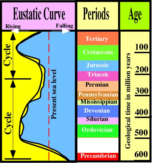
Fig. 13- The Phanerozoic 1st order eustatic cycles are linked with the Precambrian (Rodhinia or Proto-Pangea) and Permo-Triassic (Pangea) supercontinents. Assuming that water volume (in it all forms) in the Earth is constant, these 1st order eustatic cycles are directly related with the volume of oceanic basins, which is reliant to the volume of the oceanic mountains (oceanic ridges).
In spite of the time duration of these cycles has changed since the birth of sequential stratigraphy, the majority of geologists assumes the following time duration:
- 3 to 50 My(4) for 2nd order cycles,
- 0.5 to 3.0 My for 3th order cycles and
- 0.1 to 0.4 My for 4th and 5th order cycles.
The classification of eustatic cycles in different orders clearly illustrated that P. Vail and coauthors considered Eustasy as a multileveled complex geological structure in which each eustatic cycle forms a whole with respect to its parts while at same time being a part of a larger whole.
Systems thinking paradigm recognizes the existence of levels of complexity in eustasy with different kinds of laws operating at each level. At each level of complexity, i.e. at each eustatic cycle, the associated observed phenomena exhibit properties that do not exist at the lower levels. In other words, the stratigraphic cycle deposited in association with each eustatic cycle has specific properties.
Fig. 14- Assuming that the total water volume is constant since Earth formation a fast oceanic expansion induces a large volume of oceanic ridges and a sea level rise, i.e., the sea encroaches the continents. In the same way, a slow spreading induces a regression of the sea, i.e. the shorelines are displaced seaward. The amplitude of sea level changes is roughly 300 meters and the rate of oceanic expansion is around 1 cm per 1000 years (rate of nails’ growth).
Thus, during 3rd order eustatic cycles are deposited stratigraphic intervals dubbed “sequence cycles” which are often, but erroneously, considered as the fundamental “building blocks” of the stratigraphy. The term “building blocks” suggests a cartesian approach which I do not think was the Exxon's approach. Stratigraphy, as a whole, is more than the mere sum of its parts or “building blocks”(5).
The 1st order eustatic curve illustrated on plate 15 is bimodal. It shows high sea-levels during two geological intervals of time: (1) Cambro-Ordovician and (2) Late Cretaceous. These periods have long been recognized as “thallassocratic”(6) . They contrast with the widespread “epeirocratic” emergences in the latest Precambrian, Permo-Triassic, and Oligocene-Neogene times6. Each order of eustatic cycles seems to have a particular cause. Thus, the most likely cause of 1st order eustatic cycles is the tectono-eustasy, i.e. change in ocean basin volume (believed to be the related with the length of spreading ridges). In fact, the oceanic ridges are thermal bulges that displaced sea water7.
The migration of a ridge landward increases the volume of the ocean basin and induces a drop in sea level8. This argument is readily expanded. The number of lithospheric plates varies in time, and the total length of the ridges increases with the number of plates. It seems likely that the number of plates and the length of the ridge system are maximal during times of continental dispersal and minimal during times of aggregation.
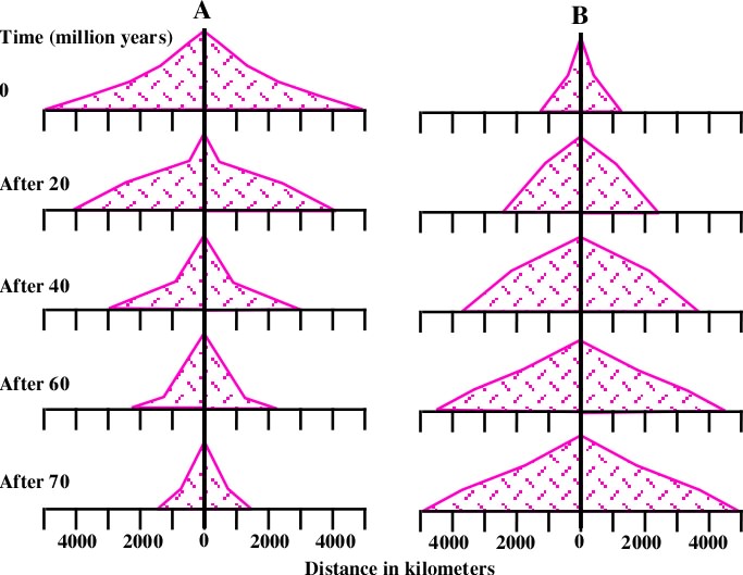
Fig.15- Profiles of fast and slow spreading mid-ocean ridges through 70 My of spreading. In example A, a ridge that had been spreading at 6 cm/y, after 70 My, has one-third of its original volume. In B, a ridge that had been spreading at 2 cm/y and changes to 6 cm/y increases the volume of the ridge.
As illustrated on fig 14, rapid spreading rates cause broad and high mid-ocean ridges. On the contrary, slow rates cause narrow and lower mid-ocean ridges.
During times of rapid sea floor spreading the ocean basins are relatively shallow and sea level rises onto continents (transgression).
During times of slow sea floor spreading the ocean basins are deeper. The seas retreat from the continents, and are restricted to the ocean basins and areas of rapid tectonic subsidence (regression).
Pitmann9 calculated the profiles of fast and slow spreading mid-ocean ridges through 70 My of spreading emphasizing the changes in the rate of sea floor spreading in eustasy (plate 17). In A, a ridge that had been spreading at 6 cm/y after 70 My, it has one-third of its original volume. Epeiric seas return to the ocean basins (regression). In B, a ridge that had been spreading at 2 cm/y changes to 6 cm/y. Such a change increases the volume of the ridge, which displacing water causes a sea level rise (transgression).
Geologists have assumed that spreading rates could change sufficiently to move sea level by some hundreds of meters. However, Cretaceous spreading rates are still imprecisely known, and those of the earlier times are probably lost beyond recall 10 &11.
Whatever relative poles might be played by change in the ridge length versus change in spreading rate, it seems clear that “plate activity” (concept that covers both factors) must have a strong influence on long term eustasy12. Nevertheless, as shown by Pitman13, such volume effects are too gradual to be the principal cause of eustatic changes of 2sd or 3rd order. They are adequate only to explain the 1st order eustatic cycles, particularly if the role of continental thickness changes, which can be regarded as an indirect response to plate activity13.
Other factors that contribute to changes in ocean basin volume are:
(i) Continental collisions, (ii) Subduction trenches, (iii) Submarine volcanism and, (iv) Sediment fill.
However, the combination of all these variables were estimated to cause a maximum rate of tectono-eustatic around 1.2 to 1.5 cm/ky3.
Second to 5th order eustatic cycles are believed to be caused by smaller magnitude, but higher frequency, and more rapid rates of eustatic change14. Such eustatic variations would cause high frequency variations on the relative change of sea level curve.
Second order eustatic cycles consist of sets of 3th order cycles. According to Vail15, a set of 5-7 third order cycles form a 2sd order cycle with a time duration averaging 5-10 My16. As we will see later, the boundaries of 2sd order eustatic cycles are characterized by particularly large eustatic falls.
Variations in volume of oceanic basins are mainly due to:
(i) the break of supercontinents and (ii) the changes on rate of sea floor spreading.
Sea level changes can also be induced by glaciations. Glaciations have an important effect on eustasy and, consequently, on the displacements of shoreline deposits. Glaciations, occur periodically at the earth's surface. They seem to be characterized by a double periodicity1 :
(i) The first one, is associated with the cyclicity of the geological periods characterized by predominant compressional tectonic regimes, i.e. periods during which the earth's surface was composed just by few lithospheric plates. In other words, when the sediments were folded and uplifted forming high mountains which are the realms of low temperatures.
(ii) The second periodicity, is independent of the structural evolution of the earth's surface. It is associated with the cyclicity of the temperature variations for which several hypothesis have been proposed.
At the earth's surface the equilibrium of the heat is controlled by the amount of sun radiation received. If two amounts of heat, L1 and L2 are received by a surface, its centesimal temperatures, T1 and T2 , are related by the equation2:
(T1+273º)/(T2+273º)= (L1 /L2)1/4
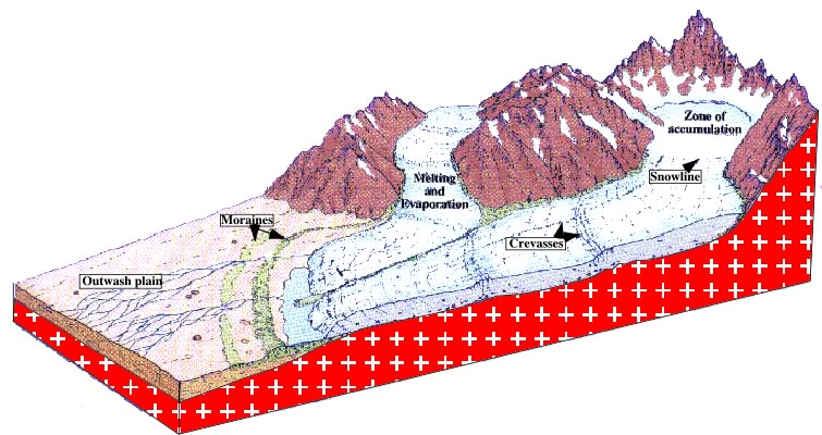
Fig. 16 – Glaciers are quite important during glaciation. The accumulation zone becomes extremely large as well as the outwash plain.
Since the Proterozoic geologists have recognized 5-6 ice ages within glaciations appeared and disappeared:
1) Proterozoic (roughly 2.700 Ma),
2) Proterozoic (roughly 2.200 Ma),
3) Precambrian (700-600 Ma),
4) Ordovician (500-400 Ma),
5) Upper Carboniferous (290 Ma),
6) Plio-Pleistocene (3-2 Ma).
The two first one took place between 2 and 3 Ga. Mounded rocks with glacial slickensides and deposits associated with glacial environments have been found, particularly in Eastern Canada. The following ice age took place during late Precambrian time, around 0.6-0.7 Ga. It seems to have affected mainly Australia, South Africa, China, Europe and North America.
After a long mild period (200 My) without ice sheets, a new ice age onset at the end of the Ordovician. After this ice age a new mild period (around 150 My) took place before the Late Carboniferous ice age (290 Ma).
The Late Carboniferous ice age was very short (20-30 My). It was partially induced by the agglutination of the Pangea. Glaciations spread in Antarctica, South America, Africa, Arabia, India and Australia.
After a period of almost 270 My of relatively mild climate the last ice age, the Cenozoic ice age, took place 2-3 Ma in the Plio-Pleistocene.
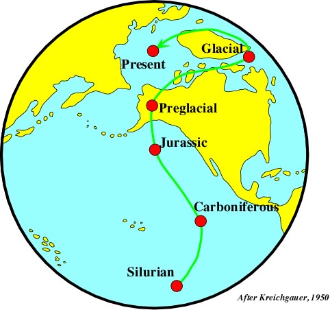
Fig. 17- This figure shows the different positions of the North Pole, since Lower Paleozoic until the present time.
The temperature of the oceans and the amount of glacial ice on the continents has a strong influence on the amount of oxy gene isotopes of seawater. Both, cooling temperatures and ice formation, change the isotope values in the same direction. Even if the two effects cannot be untangled in detail, the timing of glacial fluctuations can be very well documented3. The sudden changes occur about 35 Ma, i.e. near the Eocene-Oligocene boundary. They have been interpreted as reflecting the onset and rapid growth of continental ice cap in the Antartic4.
Before the advent of the Plate Tectonics, in order to explain the changing in climate suggested by stratigraphic studies, geologists proposed that, in the past, the position of the continents and, particularly the location of the poles, have changed5.
To explain the glaciation during the Appalachian Orogeny, in South America, South Africa, Australia and India, several geologists suggested that these areas were once agglutinated (Gondwana Continent). They located the south pole in Pacific ocean not far from Hawaii Islands. Kreichgauer6, as illustrated in fig. 17, admitted that at the begriming of Cenozoic time the North Pole traveled, firstly, toward Alaska and, then, toward South Greenland. This could explain the large ice cape between North America and North Europe. The relatively mild climate nowadays was admitted to be due to the displacement of the North Pole from South Greenland to its present day position.
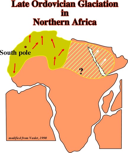
Fig. 18- This figure illustrates the probably extension of the Late Ordovician glaciation in Northern Africa and the more likely location of the South Pole. The arrows indicate the direction and sense of the ice displacement (slickensides).
When these hypotheses were advanced they were very controversial. However, in the seventies, with the advent of the Plate Tectonics, some of them were partially corroborated.
Thus, the Ordovician glaciation (400-500 Ma), for instance, is nowadays well understood. In fact, according to the Plate Tectonics paradigm, after the break-up of the Precambrian supercontinent (Proto-Pangea), Baltica and Laurentia moved northward toward the equator and the Gondwana moved polewards7. Baltica became warmer and the southern parts of Gondwana became much cooler. Few million years before the end of the Ordovician period, glaciers grew in around the south polar region of Gondwana. As the period came close, the glacial episode reached a climax and a coeval mass extinction in the marine realm took place. However, the relationships between the fauna extinction and the glaciations are speculative and controversial.
The evidence of Ordovician glacial conditions were first found in central Sahara Desert (Fig. 18). Three or four level of glacial deposits, as well as a remarkable variety of glacial features, were found. The Fig. 19, for example, illustrates the infilling of a 50 km long sinuous esker in South Sahara. This kind of deposits is one of the best hydrocarbon reservoirs in this area which development was explained by Hamblin 8, as follows:
“A glacier transports debris to ice margins. Melt water carves tunnels beneath the ice and emerges in braided streams, which deposits reworked glacial sediments on the outwash plain. In places, melt water collects along the ice margins in temporary lakes, which develop deltas and other typical shoreline features. After the ice has receded, the hummocky hills of a terminal moraine stretch in an arcuate line, conforming to the original shape of the ice margins at the farthest advance of the glacier. The retreating of glacier levees behind unsorted debris in ground moraines, and recessional moraines mark the position of the ice margin were the glacier paused during its retreat. Hills of ground moraine can be reshaped by a subsequent advance of ice, forming drumlins. Sinuous eskers remain where sediments were deposited by subglacial streams and sediments reworked by melt water form outwash-plain and lake deposits. Where ice blocks were stranded by receding glacier and partly buried under debris, the melting of ice produced kettles. Similar glacial features and less extensive ones on other parts of the continents suggest a widespreading glaciation in Ordovician time.”
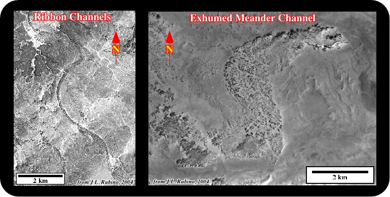
Fig. 19- In the Sahara Desert, northward of the moraines of the Late - Ordovician glaciation, that is to say, in the washout plain, long and sinuous eskers outcrop. The filling sediments are potential hydrocarbon reservoir-rocks and some of them are productive.
Others evidence of this paleozoic ice age were found in North and South America. However, several geologist consider that their age may be slightly younger, probably of Silurian. Confirmation of the age and the glacial origin of these deposits, interpreted as tillites, would indicate a continuation of the glacial episode beyond Ordovician Period. The glacial episode peaked near the close of the Ordovician and caused sea level to drop rapidly. This sea level fall and, later, the sea level rise induced by deglaciation greatly control the space available for sediments and the displacement of shoreline during the lower Paleozoic. At this point, it is important to remind here some interesting concepts proposed by Peltier9, which are fundamental to understanding sea level changes and their impact in systemic.
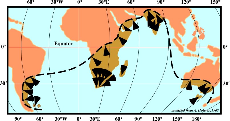
Fig 20- The extension of Lower Paleozoic glaciations and the mapping of associated slickensides strongly suggest (i) continental drifting and (ii) relatively accurate position for the South Pole at that time.
“When ice sheets melt and their melt water enter the oceans basins”... wrote Peltier ......
“we must be able to determine where in the oceans the water accumulates. Only then will it be possible to describe the differential ocean loading accurately and only then will we know how the geoidal surface is deformed. It has been conventional in the literature of glacial isostasy to answer this question in a particular simple fashion. One assumed that the added melt- water was spread uniformly over the entire surface of the oceans and the bathymetry was the same everywhere. This assumption is clearly incorrect and, in fact, leads to errors of prediction which may be significant in some locations. The reason for this is physically clear.
The equilibrium surface of the global ocean (geoid) is of necessity a surface on which the gravitational potential is constant. If for any reason the potential on this surface is locally perturbed then the resulting unbalanced gravitational force will produce current in the water which will redistribute the water mass in such away that the constancy of the surface potential will be restored. If we assume, and this is an important assumption, that during the glacial maximum at approximately 20ka BP, the ice sheets, oceans and solid Earth were in a state of gravitational (isostatic) equilibrium, then we may envision the following scenario as the ice sheets melt:
(i) Initially, the sea level is held anomalously high in the vicinity of the ice. However, everywhere on the surface of this initial ocean the gravitational potential is constant since it is in equilibrium.
(ii) When melting commences the potential on the surface is perturbed non-uniformly and the added melt water is distributed over the oceans such as to restore the potential to a new constant value everywhere.
In response to the load added over every ocean basin the sea floor will be depressed and in response to the load removed where ice sheets are mel- ting the land will be elevated. The complex redistribution of mass in the interior of the planet which is effected by the net load variation will force further irregular variations of potential on the ocean's surface and thus further redistribution of water will be required to equalize the potential. This process of continual gravitational “feedback” between the ice sheets, the oceans, and the solid earth is the process which ultimately determines the relative sea level signature which will be observed everywhere continent and sea meet”.
The Plio-Pleistocene ice age (fig. 21) and the Cenozoic glaciations in generally, were also explained by Plate Tectonics paradigm. At that time, Europe and North America were covered by a thick continental ice sheet. In North of Asia, the thickness of the ice was very thin and probably only snow had been deposited there. Such an absence of ice sheet is often associated with the non-existence of mountains in North Siberia10. This absence corroborates the hypothesis advanced by several geologists that the extension and thickness of the ice sheets are directly linked to the presence of high mountains11.
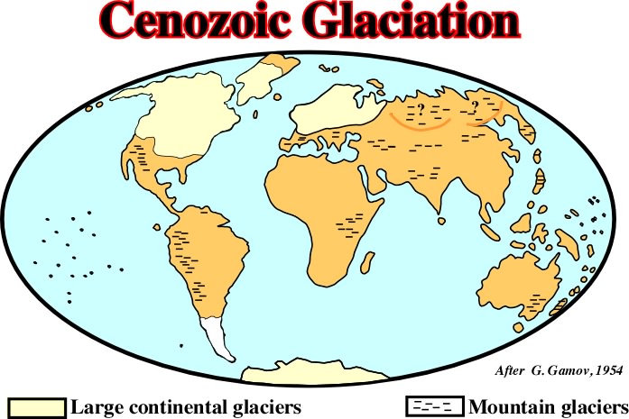
Fig. 21- Gamov (1954) proposed a mapping of the Cenozoic glaciation, in which he individualized large continental glaciers and more restricted mountain glaciers. The continental glaciers took place not only in northern Europe and North America, but in Antarctica and southern part of South America as well. The mountain glaciers developed mainly in the high areas of the Meso-Cenozoic and Paleozoic megasutures.
On the other hand, the total volume of ice deposited over the Cenozoic continents at the maximum of snowing-up should be a large number of Mkm3. As the provenance of ice was, directly or indirectly, linked with the ocean's water12, the sea level should lower than today. However, due to the large volume of oceanic ridges the volume of the oceanic basins was much smaller than today.
In fact, in spite of the glaciation, during the Cenozoic the sea-level was higher than today. Also, the continents, larger than today, under the weight of the ice continental sheets the crust subsided at least 200 meters in certain areas areas (Great Lakes and North Europe). However, since the ice melted, these areas were flooding by the rising of sea level. Marine sediments with shells and other marine fossils have been found which strongly suggests that the present day elevation is a consequence of isostatic readjustments.
Detailed studies of the Plio-Pleistocene ice age deposits indicated that, at least, four successive glacial periods (Günz, Mindel, Riss and Würm) were interrupted by relatively less cold periods known as interglacial stages. During these intermediate periods the retreat of the glaciers was much more important than today. This suggests that nowadays we are living the end of a glacial period, and before the next cold invasion the climate of North America, Europe and North Asia should grow milder.
To explain the ice ages and the sea level falls induced by glaciation, we need to find a mechanism able to reduce the amount of sun's energy received by the earth's surface. However, there is no logical reason to believe that the sun irradiated a constant amount of energy during the geological time. In addition, modern astronomic hypothesis assume that all stars, as the sun, increase the brightness with age. The calculation for the sun predicted an increase between 30 and 60 % during the last 5.000 My. On the other hand, a detailed study of sun's surface showed up the existence of important cyclic disturbances such as the sun' storms. They appear and disappear in average every 12 years and they seem to have a strong short term climate influence13.
The Proterozoic Ice Ages could be induced by the consumption of methane and ammonia of the atmosphere and the ending of the greenhouse effect which seems to be predominant during the lower Proterozoic. In the same way, the amount of different gas, volcanic particles, steam, etc., in the atmosphere, which induce important cooling due to the fact that one part of the sun energy is lost and does not reach the Earth's surface, could have contributed to the development of these ice ages (7). Nevertheless, it is very difficult to relate the volcanism and the ice ages. In fact, several geologists advanced an opposite relation. The pression of the continental ice sheets could induce volcanic activity. To make a long history short, one can say, that, so far, there is any hypothesis explaining why the volcanic activity and the ice ages should have the same rate.
With the advent of plate tectonics, geologists associated the ice ages, to the periods of large amount of continental crust. They explained the Precambrian and the Late Paleozoic ice age, by the agglutination of the Proto-Pangea and Pangea. However, such an explanation cannot be invoked to explain the other ice ages. On other hand, stratigraphic studies suggest that large glacial periods seem to be, directly, or indirectly, associated with geological periods of continental shortening and uplift.
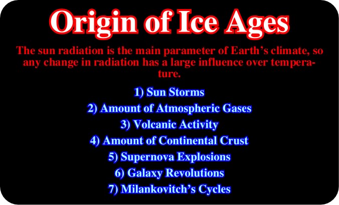
Fig. 22- The seven most likely causes of glaciations according G. Gamov.
Another invoked possible explanation of the ice ages are the Supernovas' explosions. Actually, if a supernova blew up near the earth the radiation could disrupt the earth's ozone bed and a general cooling could take place. As long and regular periods of geological time (200 My) separate the ice ages and as the solar system makes a complete galactic translation in 225 My, it was suggested that if the solar system crossed at a particular place a cosmic cloud, one fraction of the sun's radiation would be absorbed, or reflected, and only a minor fraction would reach the earth's surface with a subsequent cooling. This hypothesis explains very well the cyclicity of the ice ages, but there is any proof of such a cosmic cloud.
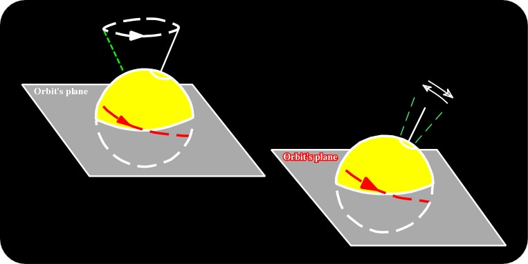
Fig. 23- The equinoxial precession, that is to say, the movement of the Earth’s axis perpendicular to the orbit’s plane (left) and the inclination of the orbit’s plane of the earth, show periodic variations (± 40My). A precession cycle is often defined as a 19 000 to 23 000 year astronomic periodicity, in full, the precession of the equinoxes (one of the three Milankovitch parameters of the Sun’s effective insolation) at the Earth’s surfaces, that gives rise to important climatic and geologic cycles, notably in sedimentation rates and composition. A second cycle, the axial precession, 25 694 years rotating in the opposite direction (clockwise), also affects climate through the ecliptic angle.
The last hypothesis invoked to explain the ice ages, or at least certain glaciations, was proposed by Milankovitch. He assumed that the main parameters controlling the sun radiation received by the earth's surface are:
(i) Precession of the earth's rotation axis.
(ii) Inclination of the orbit's plane.
(iii) Precession of the earth's orbit, and
(iv) Orbit's eccentricity.
G. Gamov's ideas 15 on this subject can be summarized as follows:
A) The earth's rotation axis moves slowly in space. It describes a cone which axis is perpendicular to the orbit's plane. This movement of the axis is known as "equinoxial precession".
Newton explained this was the result of attraction of the sun and the moon on the equatorial excrescence of the earth. It is an extremely slow movement since 26 ky are needed the earth's axis to make a complete revolution.
As this phenomenon of precession reverses periodically every 13 ky, the earth will be at the perihelion presently to the sun, alternatively, with its hemispheres North and South.
B) In addition to the ordinary precession, other perturbations of the earth's movement, due to the influence of the planets, particular that of Jupiter, are added.
The inclination of the earth's axis to the orbit's plane (which does not affect the ordinary precession) shows variations which period is more or less 40 ky.
C) The earth's orbit changes. It turns slowly around the sun and its eccentricity increases and decreases periodically.
The periods of these changes are 60 ky and 120 ky. The rotation of the earth's orbit around has the same consequences that the precession. Their effects can be added. A superperiod of the eccentricity is known. Its time lapse is around 400 ky.
D) The periodic changes of eccentricity have a big influence on the climate conditions of earth's surfaces.
During the periods of big elongation, the earth, at the ends of its trajectory, is particularly far away of the sun, and both hemispheres receive then amounts of heat abnormally lower.The calculations show that 180 ky ago the eccentricity was 2.5 times bigger than today. Such a change represents a difference in temperature of 9-10ºC between both hemispheres.
Individually, any of these causes induces substantial changes in temperature. However, if at certain time of the geological history, they are coeval, the addition of their effects can be particularly important.
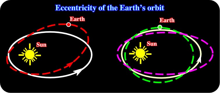
Fig. 24- The eccentricity of the earth’s orbit (orbit changing) has a big influence in the radiation received from the sun, as depicted in this figure. Indeed, the rotation of the earth‘s orbit around the sun has the same consequences as the precession. During the periods of big elongation (as in purple trajectory) the earth, at the ends, is particularly far away from the sun, subsequently both hemispheres receive amounts of heat abnormally lower. Contrariwise, a small eccentricity, particularly when combined with an opposed inclination of the earth’s axis, creates mild climatic conditions on the North hemisphere.
When the eccentricity of the orbit is particularly big, the inclination of the axis is particularly strong and the boreal summer coincides with the passage of the earth at the distal point of the orbit. The hemisphere North will be particularly cold. On the contrary, a small eccentricity combined with an opposed inclination of the axis creates on the North hemisphere, mild climatic conditions.
Shortly, astronomical events have induced an alternance of cold and mild climates during the Earth's history. However, it looks that the ice ages are particularly important during the geologic intervals characterized by predominant compressional tectonic regimes.
During such intervals, the shortening and uplifting of the sediments creates favorable topographic conditions to a cold climate develop larger glaciers. Asteroid impacts also originate cold climates, but the presence of mountains seems be required.
D - Subsidence & Accommodation
Subsidence and uplift are directly related with the tectonic regime present in a certain area, at certain geological time. Assuming an eustatic sea level constant one can say:
(1) During extensional tectonic regimes, which are characterized by a maximum effective stress (s1) vertical, sediments are lengthened. This lengthening induces subsidence. The subsidence increases the space available (accommodation), i.e. creates a relative sea level rise. Moreover, the relative sea level rise induces sedimentation.
(2) During compressional tectonic regimes, which are characterized by a maximum tectonic stress (s1) horizontal, sediments are shortened. This shortening generates uplift which decreases the accommodation (water depth) creating a relative sea fall. In turn, the relative sea level fall induces erosion.
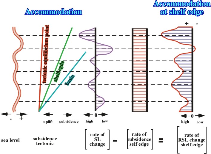
Fig. 25- The combination of eustacy and subsidence give relative sea level changes. Landward of the shelf break, a relative sea level rise increasing the space available for sediments (accommodation) favors deposition. On the contrary, a relative sea level fall decreasing the shelfal accommodation favors erosion. Seaward of the shelf break, relative sea level changes have important sedimentary consequences when the relative sea level fall is big enough to create lowstand geological conditions.
When tectonism is combined with eustatic changes the final accommodation is the sum of the that induced by tectonism and by eustasy (fig. 25). During an eustatic sea level rise (increasing of accommodation), the amount of water depth created by subsidence is added to that created by the eustatic rise. On the contrary, the amount of space created by subsidence must be subtracted by that created when the eustatic sea level falls (decreasing subsidence). In the case of an uplift, i.e. during sedimentary shortening periods, the reduction of accommodation is increased by the amount reduced by an eustatic sea level fall and decreased by the space available for the sediments created by an eustatic sea level rise.
Tectonism has the greatest effect on accommodation space. Along with climate, it controls the type and amount of sediments deposited1. Tectonism is a major control of stratigraphy, on which the tectonic events have recognizable signatures. On the basis of magnitude and duration in time, three hierarchical levels of tectonic events with typical stratigraphic signatures were distinguished by Vail2:
A) High level tectonic events
These tectonic events result from thermodynamic processes in Earth's crust and upper mantle. They are directly associated with Plate Tectonics' mechanisms. Thus, extensional rifting, sea floor spreading, tectonic sutures, compressional thrusting, etc., are considered as belonging to these long term hierarchical tectonic events. Their stratigraphic signature is the sedimentary basin. In other words, these events are the main cause of development of sedimentary basins.
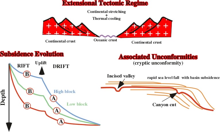
Fig. 26- Subsidence profiles can be used to classify sedimentary basins. Bally and Snelson (1980) have used the realm of subsidence to classify the sedimentary basin. In extensional tectonic regimes, rifting is associated with a differential subsidence (rift-type basin), while drifting (thermal subsidence) characterizes a continental divergent margin. Unconformities, when not tectonically enhanced are generally cryptic landward of the shelf break and in deep water.
B) Middle level tectonic events
These tectonic events occur during the evolution of the sedimentary basins, i.e. within the continental encroachment stratigraphic cycles. They may be recognized by changes in the rate of subsidence. They result from reorganization of the plate tectonics or from local thermodynamic anomalies. This class of events is characterized by a period of relatively high rate of subsidence followed by a relatively low rate of subsidence. The stratigraphic signatures are continental encroachments subcycles or major transgressive/regressive episodes, i.e. substantial downward shifts of coastal onlaps and large displacements of the shoreline.
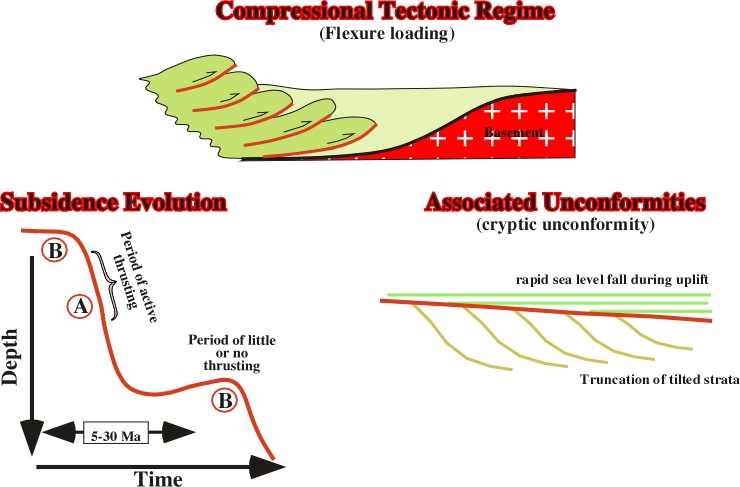
Fig. 27- In compressional tectonic regimes as for instance in foredeep basins, subsidence profiles indicate clearly the periods of strong shortening (active thrusting). The associated unconformities are tectonically enhance. However, when toplap (erosional hiatus) is not evident, they seem cryptic because onlapping is subtle.
C) Low level tectonic events
These tectonic events are folding, faulting, diapirism and magmatism activity. Their stratigraphic signatures are tilted and ruptured strata which can, often, be recognize on lower hierarchical stratigraphic cycles (sequence cycles). They are commonly associated with penecontemporanous events such as slides, slumps, megaturbidites, bentonites, datable extrusive flows and intrusive sills and dikes.
“Tectonic hierarchical events can easily be observed”..........wrote Vail3 .............“on tectonic subsidence curves constructed by plotting the depth of horizon, preferably the top of the basement, at a series of ages trough time. When the total subsidence is corrected for local isostatic compensation and sedimentary compaction, the result is a tectonic subsidence curve. Such a curve shows the water loaded hole that tectonics would create if no sediments were deposited. This is the curve to use for calculating rates and magnitudes of tectonic subsidence, assuming that isostatic compensation and compaction occur instantaneously and do not affect the subsidence of the surface deposition”.
The tectonic subsidence of a basin which evolved under extension, such as rifts and passive margins, typically shows an inflexion when the mechanism of subsidence changes from crustal extension (basin type rift) to thermal cooling (passive margin). The tectonic subsidence curves of basins that have evolved during extension are characterized by a concave upward pattern (Fig. 26). In general, they show at least two concave upward subsidence patterns. One during the crustal extension and another during the drift thermal cooling phase. However, there are additional concave upward patterns due to other crustal extension episodes, as well as thermal perturbations4.
On the tectonic subsidence curve of a basin evolving under a compressional tectonic (fig. 27) regime Vail wrote5:
“The curve shows a typically flexure loading convex upward pattern. The period of maximum thrusting is commonly associated with the maximum subsidence because this is the time when thrust sheets are building up their maximum load on the border of the foredeep basin. Several convex upward subsidence patterns are commonly present within compressional basins indicating changes in the rate of the thrust movements. There may be a period of stability or uplift between convex upward subsidence curves. The uplift may be due to the heating of the depressed crust. Transpressional basins show similar flexure loaded convex upward patterns indicating loading of a land area adjacent to the basin. Some basins were formed during an extensional regime which changed through time into an compressional regime. This change will be reflected in the basin subsidence curve, which will show a concave upward pattern in the early part, a convex upward pattern in the latter. The tectonic subsidence curve of a basin will commonly show extensional or compressional pattern. Changes in basin type will generally be apparent from the curve pattern. The tectonic subsidence curve associated with each type of sedimentary basins reflects the subsidence history of each basin, and in principle it represents the stratigraphic signature of first hierarchical level tectonic events. Each concave or convex upward pattern on the tectonic subsidence curve is generally associated with transgressive-regressive facies cycles. Transgressive-regressive facies cycles are stratigraphic signatures of changes in the rate of tectonic subsidence and are considered the signature of middle level tectonic events. Folding and faulting occur during particular periods of the tectonic subsidence curve depending on the structure type. In extensional settings faulting is most active during the crustal extension phase. In compressional settings faulting is most active in the maximum subsidence phase. A tectonic subsidence curve influenced lower level tectonic events may show a deviation from the regional subsidence pattern. For example, a tectonic subsidence curve made in a basin formed under a compressional regime will show a high corresponding to the development of a structure that is causing the flexural loading. This high will be superimposed on the regional curve that will show maximum subsidence at the corresponding time.”
The "mise in evidence" of unconformities associated with extensional and compressional tectonic regimes are quite different. In extensional regimes the unconformities are generally cryptic (fig. 26), except near the shelf break. On the contrary, in compressional regimes, the unconformities are enhanced (fig. 27). The geometrical relationships between the chronostratigraphic lines underlying and overlying the unconformity are clear and sharp. They allows an easy identification of the unconformity and its lateral picking as well.
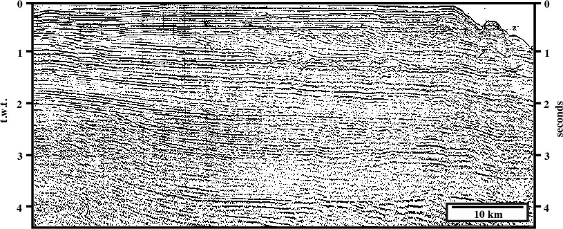
Fig. 28- On this seismic line of North America continental divergent margin, a volcanic intrusion enhanced locally a cryptic unconformity. In the upper part of the line, the forestepping interval (post-Cretaceous) is often used to illustrate the importance of the eustacy in stratigraphy, since tectonic subsidence is quite insignificant.
The seismic line illustrated in fig. 28 is representative of New Jersey offshore (Baltimore Canyon trough) which corresponds to a vertical superposition of a rift type basin and a passive margin. Extensional tectonic regimes were predominant. The subsidence through time was mainly due to crustal extension (basin type rift) and thermal cooling (passive margin). The results of COST B-2 well were used by Greenlee6 to calculate the eustatic fluctuations from stratigraphic data. The tectonic and total subsidence, the paleobathymetry, the long term sea level, as well as the more likely subsidence mechanisms proposed by Greenlee are shown in fig. 29. The total subsidence curve indicates the depth to the bottom of the well at any particular time. The tectonic subsidence is calculated by decompacting the sediments and correcting for local isostatic compensation. To obtain accurate results the subsidence curve must also be corrected for paleobathymetry and the datum adjusted to the long-term sea level curve. The tectonic subsidence curve may also be influenced by flexural loading due to the variation in thickness of adjacent sedimentary units. To separate tectonic from eustatic effects, the subsidence curve obtained can be compared with theoretically calculated subsidence curves for various amounts of crustal stretching.
From the difference between load-corrected subsidence curve and interpreted thermotectonic subsidence curve, the 1st order eustatic cycle can be estimated as discussed by Hardenbol et al.7.
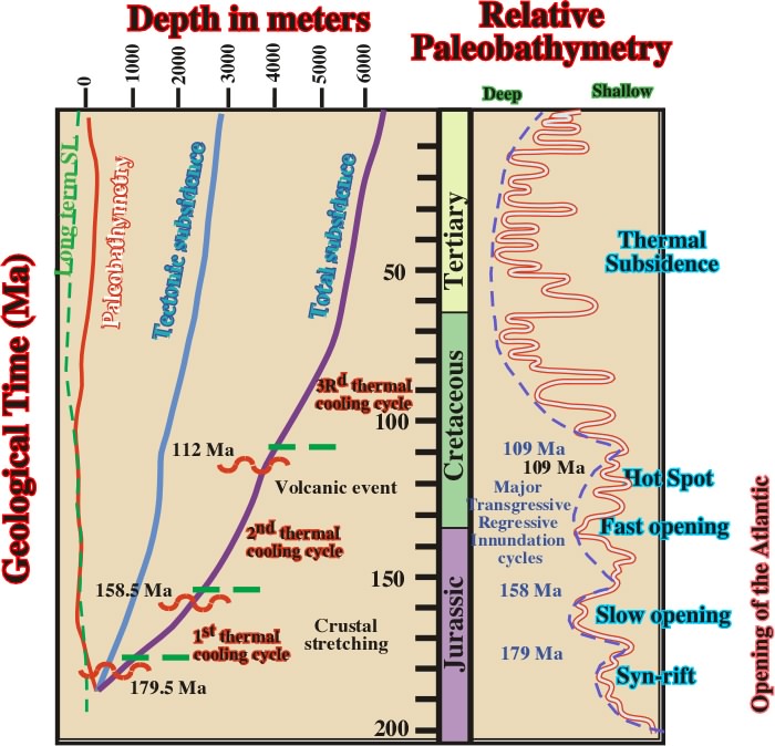
Fig. 29- Stratigraphic and tectonic events associated with the opening of North Atlantic Ocean.
On the curves illustrated in fig. 29 Vail wrote:
“It shows a relatively high rate of subsidence during the basin type rift, and is followed by a normal thermal cooling subsidence after the opening of the Atlantic, 157 Ma. During the Aptian (116-109 Ma) thermal perturbation due to an igneous intrusion resulted in slight uplift(8). Normal thermal cooling was resumed after uplift. The thermo-tectonic subsidence curve shows tectonic events of middle hierarchical level which start with in- creasing rates of subsidence. The first one extends from the late Triassic to late Jurassic (230?-157 Ma). The second one extends from late Jurassic to late Aptian (157-109 Ma) and the third from late Aptian to present (109-0 Ma). The same plate also relates the tectonic subsidence curve to variations in the paleobathymetry. Notice that there are four major transgressive-regressive facies cycles present. However, only three middle level tectonic events are visible one the thermo-tectonic subsidence curve. This is probably due to lack of stratigraphic resolution near the bottom of the well. Angular unconformities show that erosional truncation is present. They are indicated preceding the boundaries of the different stratigraphic intervals. Folding and faulting within the basin occurred during the four transgressive- regressive facies cycles. Normal faulting and other structures due to rifting were associated with the syntectonic phases of rifting, which preceded both the slow and rapid opening of the Atlantic. During the Aptian magmatic activity induced doming”.
The amount of sediments is mainly related with tectonism, eustasy and climate. As compressional tectonic regimes induce uplift they increase the amount of sediments available for deposition. Also, as eustatic and relative sea level falls disrupt the equilibrium profile of the rivers they increase the amount of sediments, since the rivers are forced to incise the ground to reach new equilibrium profiles. Climate is also an important factor not only in the carbonate deposition but in sand-shale deposition as well. As in the same basin, the terrigeneous influx changes in space and time, it is very difficult to correlate globally or, even, regionally, shoreline's displacements. This is illustrated in fig. 30, where three different situations are assumed (same RSL rise, but different terrigeneous influx).
(i) In the first situation, as the terrigeneous influx is low, the shoreline is displaced landward with a backstepping geometry. The final result is a transgression.
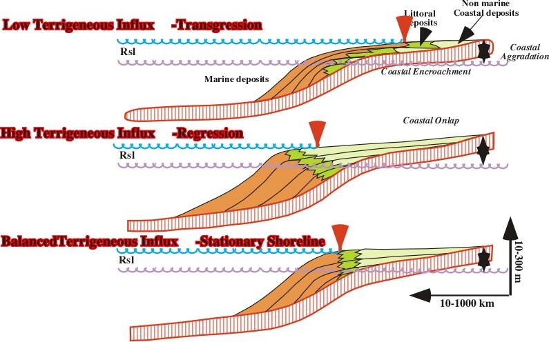
Fig. 30- Depending on terrigeneous influx, a relative sea level rise can shift the depositional coastal break landward or seaward. When the terrigeneous influx balance the accommodation the depositional coastal break remain stationary. Consequently, associating a regression or a transgression with relative a sea level change can be inaccurate.
(ii) In the second situation, as the terrigeneous influx is high, the shoreline, and associated coastal deposits, are displaced seaward. The internal configuration of the bedding planes is progradational with a strong forestepping geometry of the shoreline. The final result is a regression.
(iii) In the third situation, the terrigeneous influx is supposed to balance the accommodation induced by the relative sea level rise. The shoreline and associated deposits are stationary.
The terrigeneous influx changing laterally, particularly near the mouth of rivers, correlations of transgression / regression episodes are unlikely.
___________________________________________________________________________________
Notes (Stratigraphic Parameters), (see Bibliography) :
1 - see Vail (1989).
2 - see Suess (1888).
The original definition of eustatic movement is found in page 680: “changes which take place at approximately equal height, whether in a positive or negative direction, over the whole globe; this group we will distinguish as eustatic movements”. Suess recognized the difference between the positive and negative movements. “We are acquainted with two kinds of eustatic movements; one, produced by subsidence of the earth's crust, is spasmodic and negative; the other, caused by the growth of massive deposits, is continuous and positive (quoted by Hallam, 1992).
3 - see Macdougal (1966), pp. 117.
4 - see Vail (1977).
5 - Ibid.
A - Eustasy
1 - see Mörner (1976).
2 - Ibid.
3 - Ibid.
B - Orders of Eustatic cycles
1 - see Vail (1989).
2 - Ibid.
3 - see Vail (1977).
4 - see Fisher (1984).
5 - see Sclater (1970).
6 - see Fisher (1984), pp. 133.
7 - Ibid.
8 - see Pitmann (1978).
9 - Ibid.
10 - see Fischer (1984).
11 - Ibid.
12 - see Pitmann (1978).
13 - see Fisher (1984).
14 - see Vail (1989), pp. 10.
15 - Ibid.
16 - Ibid.
C - Glaciations (Climate)
1 - see Gamov (1956), pp. 141-143.
2 - Ibid. pp. 153.
Astronomic observations indicate that the distance to the Sun is roughly 3% smaller in December than in June. Consequently, the difference in heat received on each hemisphere is around 6%, since the radiation's intensity decrease in function of the square of the distance. Using the amount of radiation received by a surface:
(T1+273º)/(T2+273º)= (L1 /L2)1/4
one can say than in North hemisphere the summer average tem- perature is 4-5º lower, and during the winter the average temperature is 4-5º higher than in South hemisphere.
3 - see Macdoudall (1966), pp. 209.
4 - Ibid.
5 - see Gamov (1956), pp. 150.
6 - quoted in Gamov (1956).
7 - see Stanley, (1992), pp. 262.
8 - see Hamblin (1989), pp. 286.
9 - see Peltier (1980).
10 - see Gamov (1956).
11 - Ibid.
12 - Ibid.
13 - see Officer (1993), pp. 24.
14 - see Gamov (1956), pp. 151.
D - Subsidence & Accommodation
1- see Vail, (1989), pp. 5.
2 - Ibid.
3 - Ibid.
4 - Ibid
5 - Ibid.
6 - Greelee, (1989).
7 - see Hardenbol, (1987).
8- see Vail, (1989).
_______________________________________________________________
Footnotes:
(1) As said before, in this short course, systemic stratigraphy is used in place of sequence stratigraphy. However, such a change means more than a mere term replacement. I hope that you have already understood what is behind such a replacement.
(2) Chronostratigraphy in the view of Ager (1984): “is a bastard hybrid of time and rocks that serves only to obfuscate the whole record and the entire discussion. In my simple way (which perhaps only demonstrate that I am simple minded), I can see only two basic concepts in stratigraphy: one is that rocks accumulate in one way or another, and the order is that this happened during the passage of time. In other words, there are rocks, which still remain, and there is time, which has passed and can never be recovered all the rest is semantic confusion”.
(3) Glacial-eustatic and tectonic eustatic changes are often termed “truly eustatic changes”.
(4) Conventionally, My is used for a certain period of time and Ma for a geological ages. We said, the unconformity 30.0 Ma and not 30.0 My. On contrary, we can say, that these sediments were deposited in 3 My, even if they are Miocene, Cretaceous or Paleozoic.
(5) Aristotle was the first to said that “The whole is more than the sum of the parts”.
(6) Thallasocratic is the adjective of thallasocraton, i.e. a craton that is part of the oceanic crust. Epeirogenic is the adjective of epeirocraton, i.e. craton of a continental block.
(7) The volcanic clouds associated with the eruptions of Krakatoa (1906) or El Chicon (1982) had reduced, during several years, 10 to 12% of sun energy received in several Pacific's islands, such as Japan and Hawai14.
(8) This intrusion is clearly seen on the left side of the seismic line illustrated on plate 30.
to continue press
next
![]()
Send E-mail to carloscramez@gmail.com with questions or comments about this course.
Copyright © 2001 CCramez
Last modification:August, 2014