
Variations in volume of oceanic basins are mainly due to:
(i) The breakup of supercontinents ;
(ii) The changes of rates of sea floor spreading.
Sea level changes can also be induced by glaciations. Glaciations have an important effect on eustasy and, consequently, on the displacements of shoreline deposits. Glaciations occur periodically at the Earth’s surface. They seem to be characterized by a double periodicity:
(i) The first one is associated with the cyclicity of the geological periods characterized by predominant compressional tectonic regimes, that is to say, periods during which the Earth’s surface was composed just by few lithospheric plates. In other words, when the sediments were folded and uplifted forming high mountains, which are the realms of low temperatures ;
(ii) The second periodicity is independent of the structural evolution of the earth’s surface. It is associated with the cyclicity of the temperature variations for which several hypotheses have been proposed.
At the Earth’s surface the equilibrium of the heat is controlled by the amount of sun radiation received. If two amounts of heat, L1 and L2 are received by a surface, its centesimal temperatures, T1 and T2, are related by the equation:
(T1+273º) / (T2+273º) = (L1 /L2) 1/4
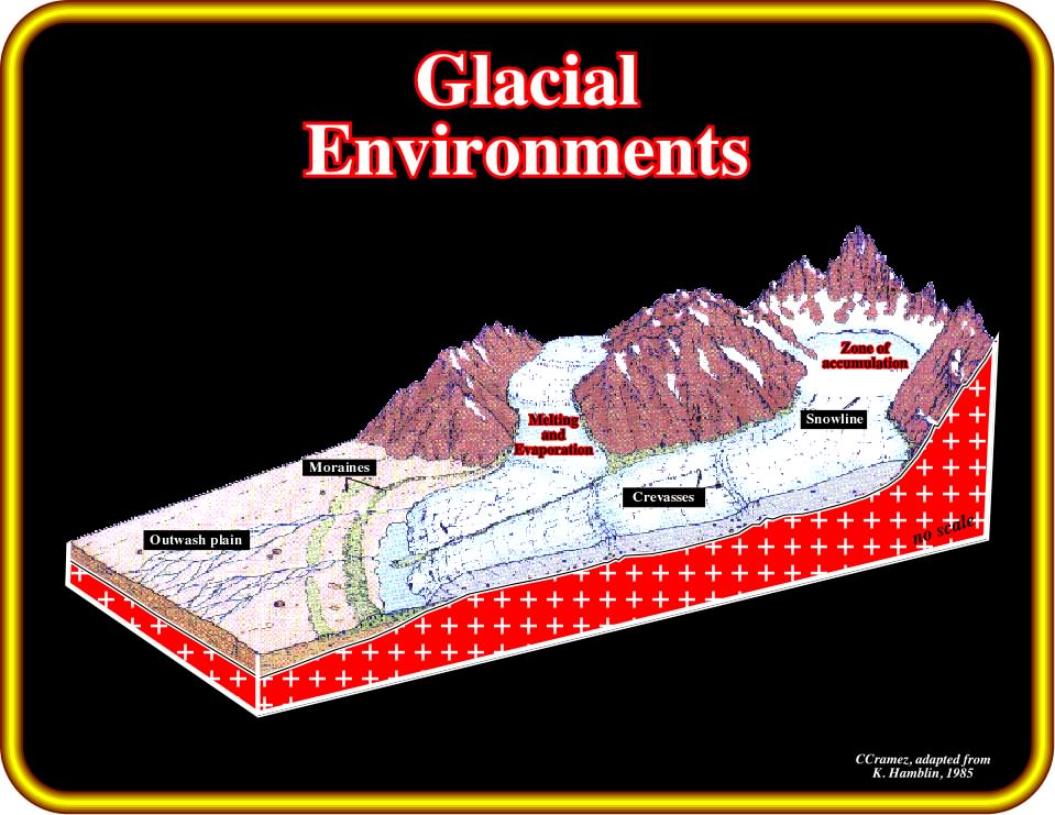
Plate 275 - As illustrated above, in a glacial environment it is important to understand the meaning of : (i) Accumulation zone (area of a glacier where mass builds up from snow faster than it is lost from evaporation or melting) ; (ii) Melting and Evaporation zone (area of a glacier where losses of ice from melting, evaporation, and sublimation exceed additions of snow annually) ; (iii) Snowline (a lower snowline indicates that more snow fell than melted, while a higher snowline indicates that less snow fell than melted) ; (iv) Crevasses (deep cracks in an ice sheet or glacier, as opposed to a crevice, which forms in rock ; they form as a result of the movement and resulting stress associated with the shear stress generated when two semi-rigid pieces above a plastic substrate have different rates of movement. (v) Moraines (any glacially formed accumulation of unconsolidated glacial debris of soil and rock, which can occur in currently glaciated and formerly glaciated regions) and (vi) Outwash plain or sandur (is a plain formed of glacial sediments deposited by meltwater outwash at the terminus of a glacier). Glaciers are quite important during glaciation periods, during which, the accumulation zone is extremely large and the snow line quite low, as well as the outwash plain. The relationships between long-term sea level changes, climate, volcanism and biotic crises have been quite well established by Fischer (1983), as depicted above.
Since the Proterozoic, geoscientists have recognized six major ice ages within glaciations appearing and disappearing:
(i) Proterozoic (roughly 2.7 Ga) ;
(ii) Proterozoic (roughly 2.2 Ga) ;
(iii) Precambrian (700-600 Ma) ;
(iv) Ordovician (500-400 Ma) ;
(v) Upper Carboniferous (290 Ma) ;
(vi) Plio-Pleistocene (3-2 Ma).
- Proterozoic glaciations took place between 2 and 3 Ga. Mounded rocks with glacial slickensides and deposits associated with glacial environments have been found, particularly in Eastern Canada.
- The second ice age took place during Late Precambrian time, around 0.6-0.7 Ga. It seems to have affected mainly Australia, South Africa, China, Europe and North America.
- After a long mild period (200 My) without ice sheets, a new ice age began at the End of the Ordovician. Then a new mild period (around 150 My) took place before a Late Carboniferous ice age (290 Ma).
- The Late Carboniferous ice age was very short (20-30 My). It was partially induced by the agglutination of Pangea. Glaciations spread in Antarctica, S. America, Africa, Arabia, India and Australia.
- After a period of almost 270 My of relatively mild climate, the last ice age was Cenozoic. It took place between 2 and 3 Ma in Plio-Pleistocene.
The temperature of the oceans and the amount of glacial ice on the continents, has a strong influence on the amount of oxygen isotopes of seawater. Both cooling temperatures and ice formation change the isotope values in the same sense. Even if the two effects cannot be untangled in detail, the timing of glacial fluctuations can be very well documented by using isotopic analysis.
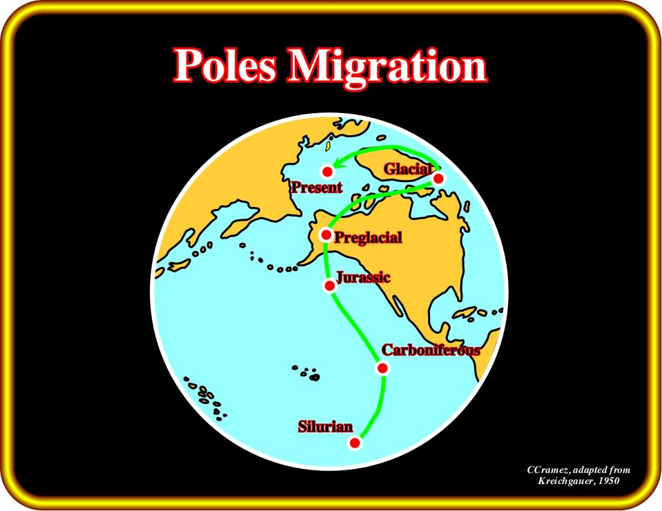
Plate 276 - This sketch depicts the different positions of the North Pole since Lower Paleozoic till present time. During the Lower Paleozoic, it was localized in the lower Pacific ; in the Carboniferous, it was localized near the equator, while in Jurassic time, it was localized roughly at the latitude of Vancouver. In the pre-glacial age, the North Pole was localized in Alaska, while during the glacial age it was located between south Greenland and Baffin Island. Comparing this plate with plate 277 (Late Ordovician Paleogeography proposed by Scotese), it is quite evident that the poles are more or less in a fixed position, but the continents move a lot function of plate tectonics (Earth's outer layer is made up of plates, which have moved throughout Earth's history, which explains the how and why behind mountains, volcanoes, and earthquakes, as well as how, long ago, similar animals could have lived at the same time on what are now widely separated continents).
The temperature of the oceans and the amount of glacial ice on the continents has a strong influence on the amount of oxygen isotopes of seawater. Both cooling temperatures and ice formation, change the isotope values in the same sense. Even if the two effects cannot be untangled in detail, the timing of glacial fluctuations can be very well documented.
Sudden changes occurred about 35 Ma, that is to say, near the Eocene-Oligocene boundary. They have been interpreted as reflecting the onset and rapid growth of continental ice caps in the Antarctic. Before the advent of Plate Tectonics, in order to explain the change in climate suggested by stratigraphic studies, geologists thought that in the past the position of the continents and particularly the location of the poles, had changed.
To explain the glaciation during the Appalachian Orogeny, in South America, South Africa, Australia and India, several geoscientists suggested that these areas were once agglutinated (Gondwana Continent). Function of the movement of the lithospheric plates, on can say that in relation to the present position of the continents, that the South Pole (see Plate 279) was in the Pacific Ocean, not far from the Hawaii Islands. Similarly, Kreichgauer (1950), as depicted on Plate 276, admitted that at the beginning of Cenozoic time the North Pole traveled, firstly, toward Alaska and, then toward South Greenland. This could explain the large ice cape between North America and North Europe. The relatively mild climate nowadays was admitted to be due to the displacement of the North Pole from South Greenland to its present day position.
When these hypotheses were advanced they were very controversial. However, in the seventies, with the advent of Plate Tectonics, some of them were partially corroborated:
- Thus, the Ordovician glaciation (400-500 Ma), for instance, is nowadays well understood. In fact, according to the Plate Tectonics paradigm, after the breakup of the Precambrian supercontinent (Proto-Pangea or Rodhinia), Baltica and Laurentia moved northward toward the equator and the Gondwana moved polewards. Baltica became warmer and the southern parts of Gondwana became much cooler.
- A few million years before the end of the Ordovician period, glaciers grew in around the south polar region of Gondwana. As the period came to a close, the glacial episode reached a climax and a coeval mass extinction in the marine realm took place. However, the relationships between the fauna extinction and the glaciations are speculative and controversial. The evidence of Ordovician glacial conditions was first found in the central Sahara Desert (Plate 277 and 278), where three or four level of glacial deposits, as well as a remarkable variety of glacial features, were discovered.
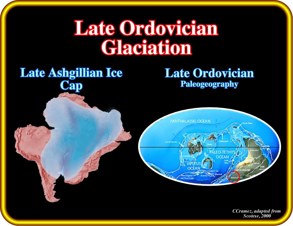
Plate 277 - The probable extension of the Late Ordovician glaciation is illustrated on the left. The geometry of the late Ashgillian ice cap allows the prediction of the more likely location of the South Pole. The map on the right illustrates, according Scotese, the paleogeography of the late Ordovician, during which, glacial sediments were deposited, as illustrated in Plate 278.
On Plate 278, for instance, is illustrated the silting up of a 50 km long and sinuous esker in South Sahara. This kind of glacial deposit, which is one of the best hydrocarbon reservoir-rocks in northern Africa, can be explained as follows (Hamblin, 1989):
“A glacier transports debris to ice margins. Meltwater carves tunnels beneath the ice and emerges in braided streams, which deposits reworked glacial sediments on the outwash plain. In places, meltwater collects along the ice margins in temporary lakes, which develop deltas and other typical shoreline features. After the ice has receded, the hummocky hills of a terminal moraine stretch in an actuate line, conforming to the original shape of the ice margins at the farthest advance of the glacier. The retreating of glacier leaves behind unsorted debris in ground moraines, and recessional moraines mark the position of the ice margin where the glacier paused during its retreat. A subsequent advance of ice, forming drumlins, can reshape hills of ground moraine. Sinuous eskers remain where subglacial streams deposited sediments and sediments reworked by melt-water form outwash plain and lake deposits. Where ice blocks were stranded by receding glaciers and partly buried under debris, the melting of ice produced kettles. Similar glacial features and less extensive ones on other parts of the continents suggest a wide spread glaciation in Ordovician time.”
Others evidence of this Paleozoic ice age was found in North and South America. However, several geologists consider that their age may be slightly younger, probably Silurian. Confirmation of the age and the glacial origin of the associated deposits, interpreted as tillites, would indicate a continuation of the glacial episode beyond the Ordovician Period. The glacial episode peaked near the close of the Ordovician and caused sea level to drop rapidly. This sea level fall and, later, the sea level rise induced by deglaciation greatly controlled the space available for sediments and the displacement of shorelines during the lower Paleozoic.
At this point, it is important to remind here some interesting concepts proposed by Peltier (1980), which are fundamental to understanding sea level changes and their impact in sequential interpretation.
- When ice sheets melt and their meltwater enter the oceans basins, we must be able to determine where in the oceans the water accumulates. Only then, will it be possible to describe the differential ocean loading accurately and, only then, will we know how the geoidal surface is deformed. It has been conventional in the literature of glacial isostasy to answer this question in a particular simple fashion. One assumed that the added meltwater was spread uniformly over the entire surface of the oceans and the bathymetry was the same everywhere. This assumption is clearly incorrect and, in fact, leads to errors of prediction, which may be significant in some locations. The reason for this is physically clear.
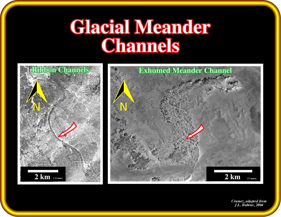
Plate 278- In the Sahara Desert, northward of the moraines of the Late-Ordovician glaciation, i.e., in the washout plain, long and sinuous eskers outcrop (long winding ridge of stratified sand and gravel with a geoemtry simila to railway embankments). In favorable geological conditions, the filling sediments forming the eskers can be are potential hydrocarbon reservoir-rocks (Algeria onshore) and some of them are productive.
The equilibrium surface of the global ocean (geoid) is of necessity a surface on which the gravitational potential is constant. If for any reason, the potential on this surface is locally perturbed then the resulting unbalanced gravitational force will produce a current in the water, which will redistribute the water mass in such a way that the constancy of the surface potential will be restored. If we assume, and this is an important assumption, that during the glacial maximum at approximately 20 ka BP, the ice sheets, oceans and solid Earth were in a state of gravitational (isostatic) equilibrium, then we may envision the following scenario as the ice sheets melt:
(i) Initially, the sea level is held anomalously high in the vicinity of the ice. However, everywhere on the surface of this initial ocean the gravitational potential is constant since it is in equilibrium.
(ii) When melting commences the potential on the surface is perturbed non-uniformly and the added meltwater is distributed over the oceans such as to restore the potential to a new constant value everywhere.
In response to the load added over every ocean basin the sea floor will be depressed and in response to the load removed where ice sheets are melting the land will be elevated. The complex redistribution of mass in the interior of the planet, which is effected by the net load variation, will force further irregular variations of potential on the ocean‘s surface and thus further redistribution of water will be required to equalize the potential. This process of continual gravitational “feedback” between the ice sheets, the oceans, and the solid earth is the process which ultimately determines the relative sea level signature, which will be observed everywhere continent and sea meet”
The Paleozoic ice age (Plate 279) and the Cenozoic glaciations, in generally, can be explained by Plate Tectonics paradigm. At that time, a thick continental ice sheet covered Europe and North America. In north of Asia, the thickness of the ice was very thin and probably only snow had been deposited there. The absence of an ice sheet is explained as due to the non-existence of mountains in North Siberia. This corroborates the hypothesis advanced by several geologists that the extension and thickness of the ice sheets are directly linked to the presence of high mountains.
The total volume of ice deposited over the Cenozoic continents, at the maximum of snowing-up, should be a large number of Mkm3. The provenance of ice was, directly or indirectly, linked with the ocean’s water. The sea level should have been lower than today. Due to the large volume of oceanic ridges, the volume of the oceanic basins was much smaller than today. In spite of the glaciation, during the Cenozoic the sea level was higher than today. The continents, larger than today, under the weight of the ice continental sheets subsided, in certain areas, at least 200 metes (Great Lakes and North Europe). Since the ice melted, these areas were flooded by rising sea level.
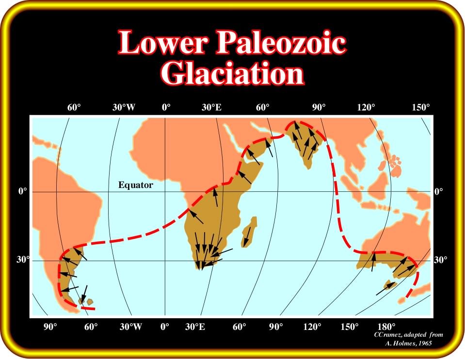
Plate 279 - The extension of Lower Paleozoic glaciations and the mapping of associated slickensides strongly suggest (i) continental drifting and (ii) a relatively accurate position of the South Pole at that time. Indeed, a palinspastic reconstitution, not only gives a rough geometry of Pangea but also the more likely location of the South Pole at Lower Paleozoic time.
Marine sediments with shells and other marine fossils have been found. They strongly suggest the present day sea level elevation is a consequence of isostatic readjustments. Detailed studies of the Plio-Pleistocene ice age deposits indicate that at least four successive glacial periods:
(i) Günz ; (ii) Mindel ; (iii) Riss ; (iv) Würm
were interrupted by relatively less cold periods known as interglacial stages. During these intermediate periods the retreat of the glaciers was much further than today. This suggests that nowadays we are living at the end of a glacial period, and before the next cold invasion, the climate of North America, Europe and North Asia should grow milder.
To explain the ice ages and sea level falls induced by glaciation, we need to find a mechanism able to reduce the amount of sun‘s energy received by the earth’s surface. There is no logical reason to believe that the sun radiated a constant amount of energy during geological time. Modern astronomic hypothesis assume that all stars, as the sun, increase brightness with age. The calculation for the sun predicts an increase between 30 - 60 % during the last 5000 My.
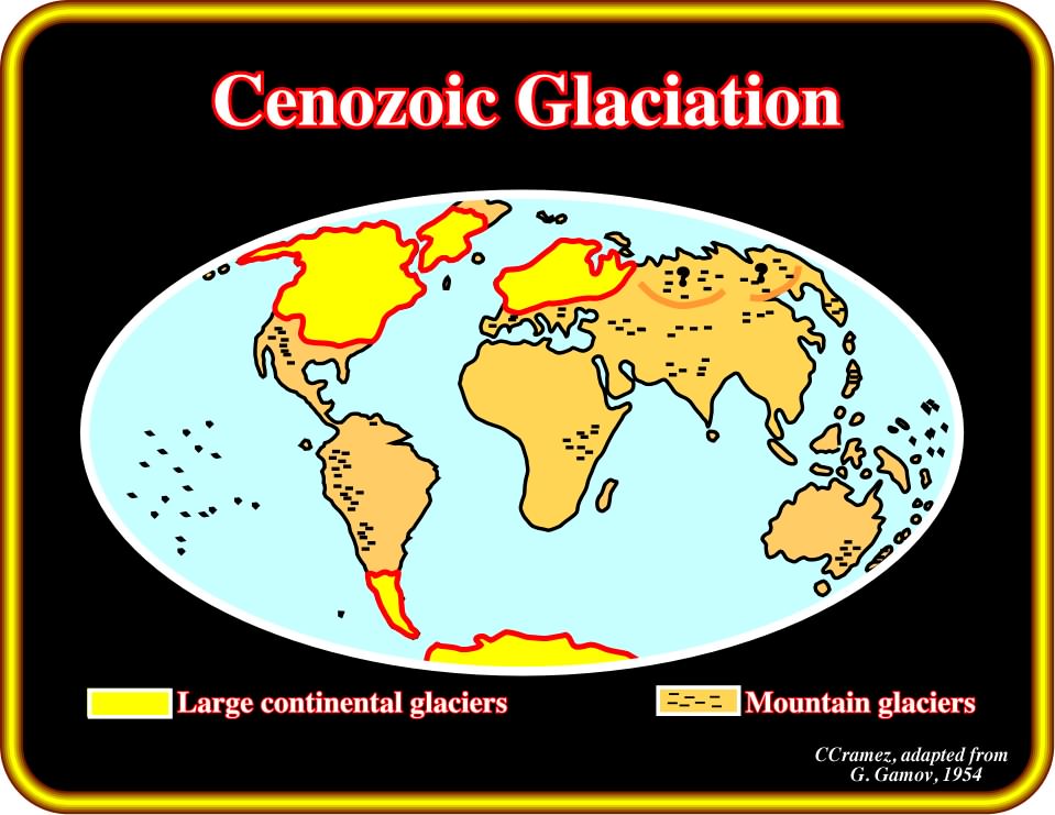
Plate 280 - On this map of the Cenozoic glaciation proposed by Gamov (1954), he individualized large continental glaciers and more restricted mountain glaciers. The continental glaciers took place not only in northern Europe and North America, but in Antarctica and southern part of South America as well. The mountain glaciers developed mainly in high areas of the Meso-Cenozoic and Paleozoic megasutures.
A detailed study of sun‘s surface showed the existence of important cyclic disturbances (e.g. sun’ storms):
- They appear and disappear on average every 12 years ;
- They seem to have a strong short-term climate influence.
On the other hand:
- The consumption of methane and ammonia of the atmosphere and the ending of the greenhouse effect, which seems to be predominant during the Lower Proterozoic, can explain Proterozoic Ice Ages.
- The amount of different gas, volcanic particles, steam, etc., in the atmosphere, which induce important cooling due to the fact that one part of the sun’s energy is lost and does not reach the Earth‘s surface, could have contributed to the development of these ice ages.
- It is very difficult to relate volcanism and ice ages (see Plate 281). Several geologists advanced an opposite relation; the pressure of the continental ice sheets could induce volcanic activity.
To make a long history short, one can say, that so far, there is no hypothesis explaining why volcanic activity and ice ages should have the same rate. With the advent of plate tectonics, geologists associated the ice ages to periods with large amount of continental crust. They explained the Precambrian and the Late Paleozoic ice ages due to the agglutination of Proto-Pangea (Rodhinia) and Pangea. However, such an explanation cannot be invoked to explain the other ice ages. On the other hand, stratigraphic studies suggest that large glacial periods seem to be, directly, or indirectly, associated with geological periods of continental shortening and uplift.
Another invoked possible explanation of the ice ages is supernovas' explosions. If a supernova blew up near the earth the radiation could disrupt the earth’s ozone bed and a general cooling could take place, as long and regular periods of geological time (200 My) separate the ice ages and as the solar system makes a complete galactic translation in 225 My.
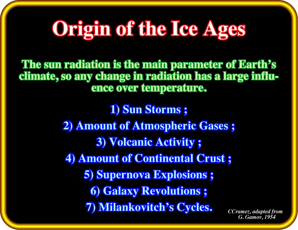
Plate 281 - According to G. Gamov (1950), the above seven causes are the most likely causes of glaciations. Although the Sun is a calm star than other stars in the universe, it still has several forms of violent storms that occur often in sun's atmosphere. These include prominences, solar flares, solar wind, and sunspots. Supernova explosion occur when a stronger star sucksthe fuel of a nearby smaller star.
It was suggested that if the solar system crossed at a particular place a cosmic cloud, one fraction of the sun‘s radiation would be absorbed, or reflected, and only a minor fraction would reach the earth’s surface with a subsequent cooling. This hypothesis explains very well the cyclicity of the ice ages, but there is no proof of such a cosmic cloud. The last hypothesis to explain the ice ages, or at least certain glaciation, was proposed by Milankovitch. He assumed the main parameters controlling the sun radiation received by the earth‘s surface are:
(i) Precession of the earth’s rotation axis ;
(ii) Inclination of the orbit‘s plane ;
(iii) Precession of the earth’s orbit ;
(iv) Eccentricity of the earth’s orbit.
On this subject G. Gamov’s ideas can be summarized as follows:
A) The earth‘s rotation axis moves slowly in space. It describes a cone which axis is perpendicular to the orbit’s plane (Plate 282). This movement of the axis is known as “equinoxial precession”.
- Newton explained that this was the result of attraction of the sun and the moon on the equatorial excrescence of the earth. It is an extremely slow movement. It makes a complete revolution in 26000 years. As the phenomenon of precession reverses periodically every 13000 years, the Earth will be at the perihelion presently to the sun, alternatively, with its hemispheres North and South.
B) In addition to ordinary precession, other perturbations of the Earth‘s movement, due to the influence of the planets, particular that of Jupiter, are added.
- The inclination of the earth’s axis to the orbit‘s plane (which does not affect the ordinary precession) shows variations in period of more or less 40 ky.
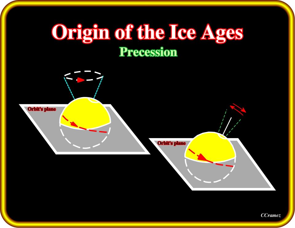
Plate 282- The equinoxial precession, that is to say, the movement of the Earth’s axis perpendicular to the orbit’s plane (left) and the inclination of the orbit’s plane of the earth, show periodic variations (± 40My). A precession cycle is often defined as a 19 000 to 23 000 year astronomic periodicity, in full, the precession of the equinoxes (one of the three Milankovitch parameters of the Sun’s effective insolation) at the Earth’s surfaces, that gives rise to important climatic and geologic cycles, notably in sedimentation rates and composition. A second cycle, the axial precession, 25 694 years rotating in the opposite direction (clockwise), also affects climate through the ecliptic angle.
C) The earth’s orbit changes. It turns slowly around the sun. Its eccentricity increases and decreases periodically.
- The periods of these changes are 60 ky and 120 ky.
- The rotation of the earth‘s orbit has the same consequences as the precession.
- Their effects can be added.
- A superperiod of the eccentricity is known. Its time lapse is around 400 ky.
D) The periodic changes of eccentricity have a big influence on the climate conditions of earth’s surfaces (Plate 283).
During periods of big elongation, the earth, at the ends of its trajectory, is particularly far away from the sun. Both hemispheres receive amounts of heat abnormally lower. Calculations show that 180 ky ago the eccentricity was 2.5 times bigger than presently. This change represents a difference in temperature of 9 to 10º C between both hemispheres.
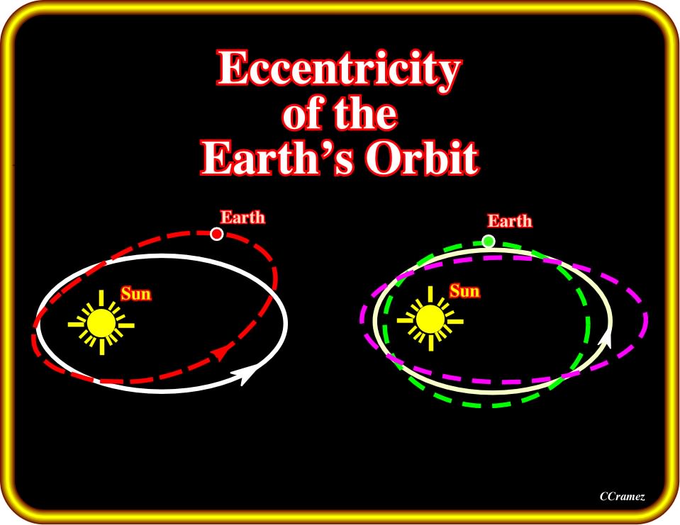
Plate 283 - The eccentricity of the earth’s orbit (orbit changing) has a big influence in the radiation received from the sun, as depicted in this plate. Indeed, the rotation of the earth‘s orbit around the sun has the same consequences as the precession. During the periods of big elongation (as in purple trajectory) the earth, at the ends, is particularly far away from the sun, subsequently both hemispheres receive amounts of heat abnormally lower. Contrariwise, a small eccentricity, particularly when combined with an opposed inclination of the earth’s axis, creates mild climatic conditions on the North hemisphere. The eccentricity of the Earth's orbit is currently about 0.0167; the Earth's orbit is nearly circular. Over hundreds of thousands of years, the eccentricity of the Earth's orbit varies from nearly 0.0034 to almost 0.058 as a result of gravitational attractions among the planets.
Individually, any of these causes induces substantial changes in temperature. However, if at a certain time of geological history, they are coeval, the addition of their effects can be particularly important. When the eccentricity of the orbit is significantly big, the inclination of the axis is particularly strong. The boreal summer coincides with the passage of the earth at the distal point of the orbit. The North hemisphere will be particularly cold. Contrariwise, a small eccentricity combined with an opposed inclination of the axis creates mild climatic conditions on the North hemisphere.
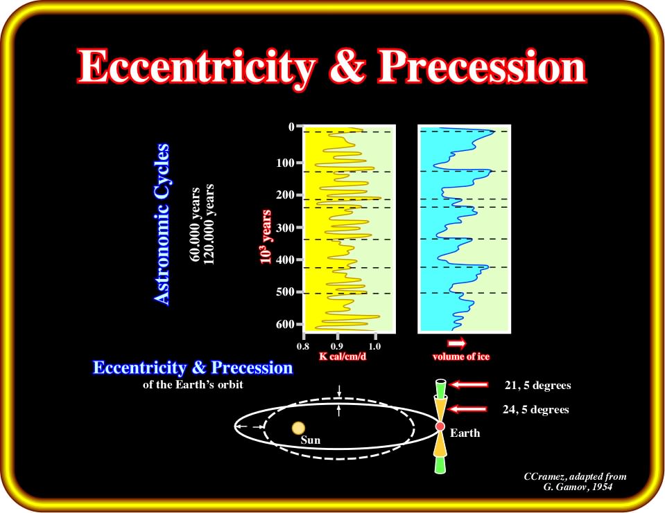
Plate 284 - It is quite evident that astronomic cycles have a great influence on the solar energy received by the earth. As illustrated above, the correlation between the volume of ice on the earth and the heat energy received from the sun is quite good (correlation does necessarilly means causation). Two major cycles, around 60 ky and 120 ky, are easily be recognized. The time scale of these graphics is too small and so the well known super-cycles, with a time duration of 400 ky, cannot be recognized. When eccentricity and precession play in the same sense, the addition of their effects can be particularly important. Astrology, that is to say, the belief systems which hold that there is a relationship between astronomical phenomena and events in the human world, is just a financial applications of astronomic cycles
To sum up:
Astronomer Milutin Milankovitch calculated a curve of the intensity of solar radiation on the ground at latitude 65° according to three characteristics of the Earth's rotation around the sun: (1) the variation of the eccentricity of Earth's orbit around the Sun, (2) the change in the tilt of Earth's rotation axis to the plane of the ecliptic and (3) the precession of the equinoxes. In the Milankovitch model, the solar output is constant and the variation of solar intensity to latitude 65° depends only on the Earth - Sun distance and angle of exposure. The addition of these three astronomical cycles (22,000 years, 41,000 years and 100,000 years) produced the curve of oscillations of the intensity of solar radiation which controls the Earth's climate, the geological time scale.
Astronomical events have induced an alternate of cold and mild climates during the Earth‘s history. However, it seems that the ice ages are particularly marked during the geologic intervals characterized by predominant compressional tectonic regimes. During such intervals, the shortening and uplifting of sediments creates favorable topographic conditions to a cold climate for developing larger glaciers. Asteroid impacts also originate cold climates, but the presence of mountains seems to be required.
to continue press![]()
![]()