The stratigraphic model proposed by the Exxon team assumes that:
“Eustasy is the main factor driving the cyclicity of sedimentary deposits”
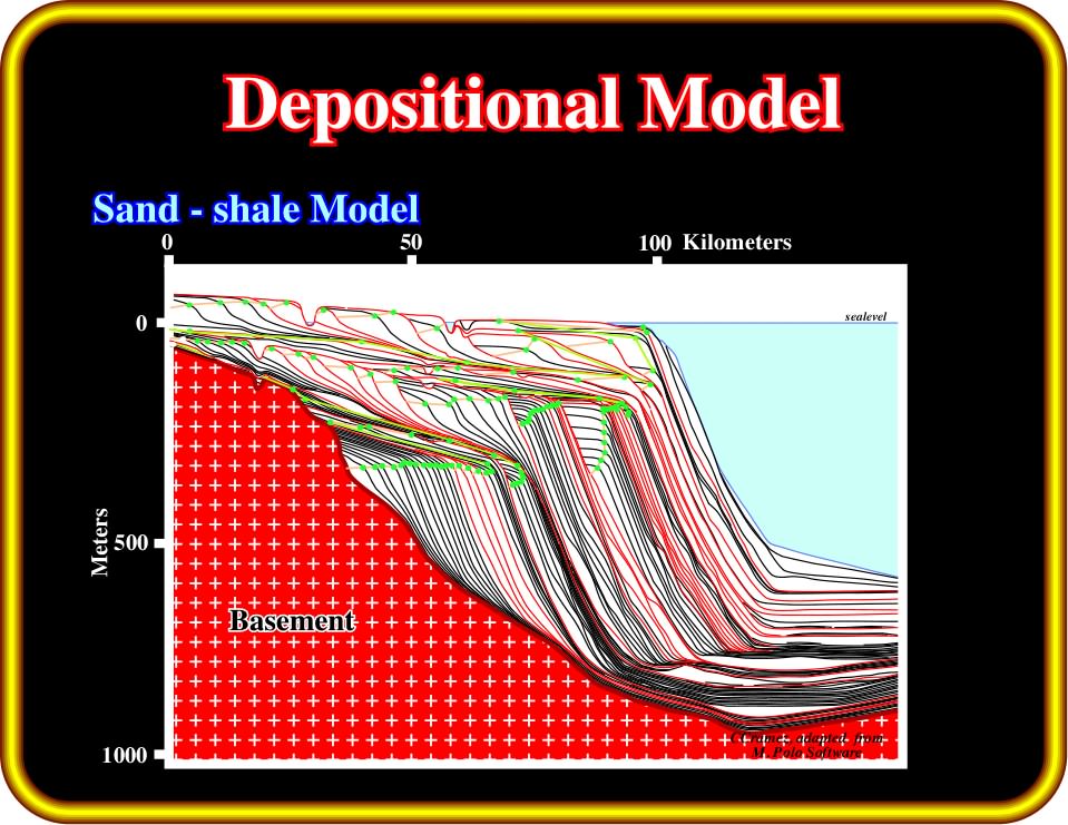
Plates 309 and 311 illustrate the classical sand-shale depositional model proposed by P. Vail and coauthors using Marco Polo software (1991).
Plate 309- Exxon’s sequence-cycle model is here represented using Marco Polo software. The vertical and horizontal scales are quite different. The vertical scale is metric. The horizontal is kilometric. The vertical exaggeration is almost 100 times. Each line corresponds to a chronostratigraphic line. Their spacing is 100 ky. The red lines correspond to unconformities, i.e., to relative sea level falls. The green dots underline the successive positions of the shelf breaks. In this model, the terrigeneous influx is constant, that is to say, the area between the consecutive chronostratigraphic lines is constant.
In this model the main geological parameters affecting the stratal patterns are assumed to be:
a) Eustasy ;
b) Subsidence ;
c) Accommodation ;
d) Terrigeneous influx ;
e) Climate.
They clearly emphasize that Stratigraphy to P. Vail is systemic, i.e., global. All parameters are interconnected and interdependent. Their interconnections corroborate the scientific “systems thinking” approach and Lovelock‘s Gaia hypothesis as well.
Several simplifications were used in this model (Plate 309), which attempts to explain the cyclicity and stratal patterns of sand-shale sedimentary intervals as recognized in the field, subsurface and seismic data:
1- A climate and a terrigeneous influx devoid of carbonate deposition ;
2- A constant (in time and space) terrigeneous influx ;
3- A gradual and linear basinward increasing of subsidence;
4- A 100 ky time interval between each chronostratigraphic line ;
5- An aleatoric location of erosion features (incised valleys, canyons, etc.) during the major relative sea level falls.
These simplifications obey the Occam’s razor. They follow the principle used by P. Bak (1996):
“Observing details may be entertaining and fascinating but, in fact, we learn from generalities”
On the other hand, it is very important never forget that:
(i) A seismic line is a representation of the subsurface. Remember R. Magritte's purpose when he named his work of art “This is not a pipe” was to express the difference between “being” and “representing”.
(ii) All geological structures are scale invariant. They cannot be correctly interpreted without a scale.
In Plates 309 to 311, the vertical and horizontal scales are different. They are both metric. However, they are quite different. The vertical exaggeration is almost 100 times the natural scale (1:1), as it exists in nature, that is to say, without magnification or reduction.
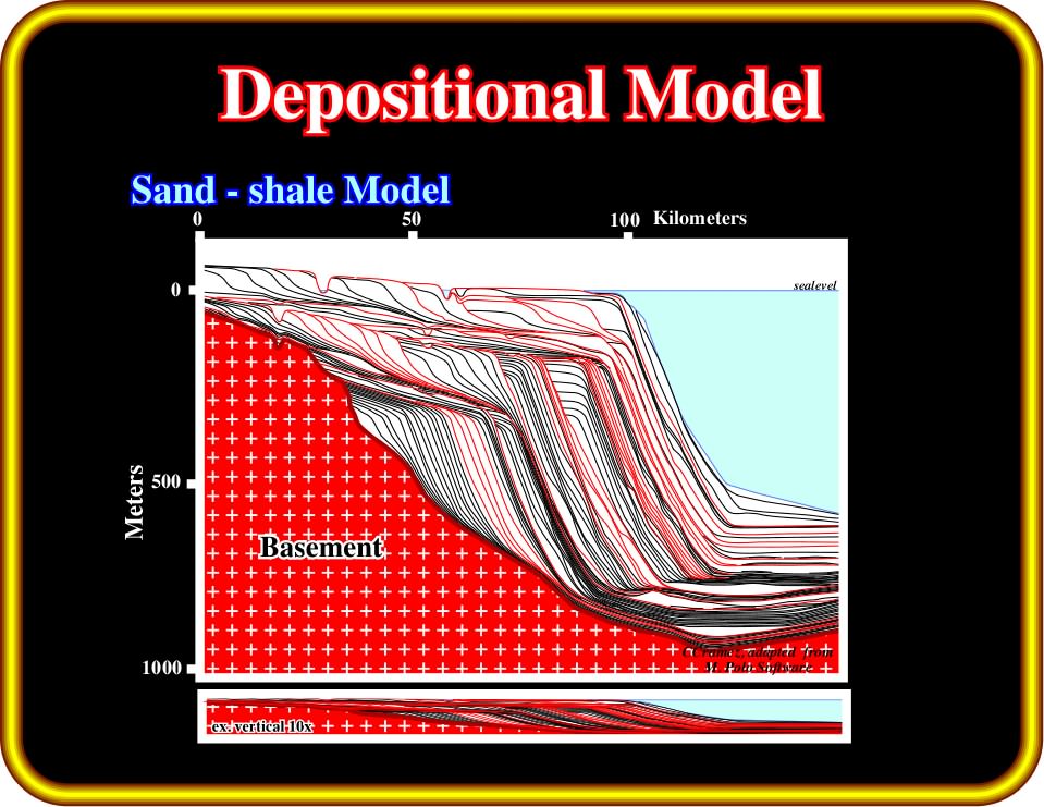
Plate 310- Exxon’s model is here represented at two different vertical scales. In the lower part, the model still is 10x vertically exaggerated. However, the majority of the geometric relationships between the chronostratigraphic lines (or reflection terminations) cannot be recognized. Taking into account that the vertical exaggeration of a normal seismic line (time profile) ranges between 2 and 3, it is evident that seismic interpretations at the level of sequence-cycles are only possible in areas with high depositional rates.
With such an exaggerated model, the geometrical relationships between chronostratigraphic lines (bedding planes) are quite evident:
- Onlap:
A base-discordant relation in which initially horizontal strata terminate progressively against an initially inclined surface, or in which initially inclined strata terminate progressively up-dip against a surface of greater initial inclination.
- Downlap:
A base-discordant relation in which initial inclined strata terminate downdip against an initially horizontal or inclined surface.
- Toplap:
Termination of strata against an overlying surface as a result of nondeposition (sedimentary bypassing) with perhaps only minor erosion. Each unit of strata laps out in a landward direction at the top of the unit, but the successive terminations lie progressively seaward.
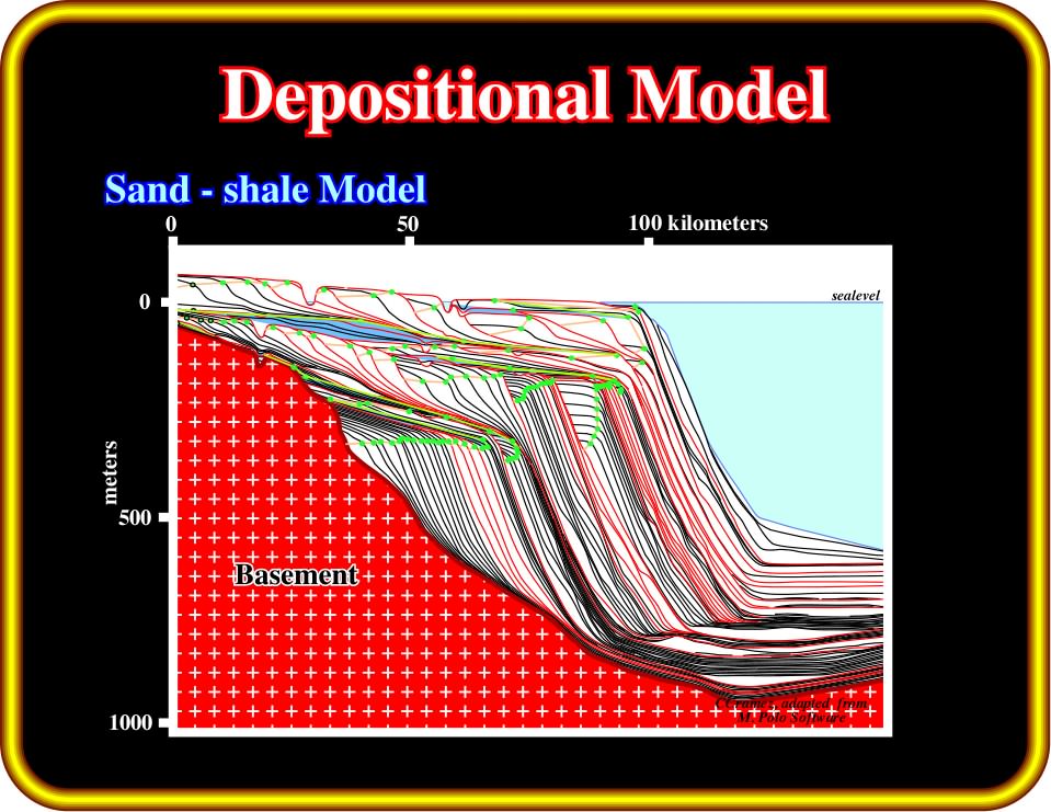
Plate 311- During regressive (forestepping) periods, the sedimentary basins have no platforms. Shelf breaks and the depositional coastal breaks (roughly the shoreline) are coincident. Platform or shelf environments are developed during transgressive periods as a consequence of backstepping of depositional coastal breaks and subsequent progressive formation of platform (depth water less than 200 meters). As during transgressive episodes the shoreline, progressively, moves landward, the water depth of the platform increases.
When Exxon’s model is drawn at natural scale (1:1) or, even, with vertical exaggerations between 5 and 10 times, most of the geometrical relationships (or reflection terminations) cannot be recognized (Plate 310). This feature raises several questions:
1) Under what conditions, can the Exxon sand-shale model be used in the interpretation of conventional seismic lines, knowing that the vertical time scale, when converted in depth, has vertical exaggerations ranging between 2 and 10 times?
2) Are sea level changes the major factor of sedimentary cyclicity and the cause of discontinuities (unconformities) bounding the stratigraphic cycles?
3) Is the Exxon basic stratigraphic hypothesis valid in all sedimentary basins?
4) Are the rates of subsidence and terrigeneous influx smaller than the rates of sea level changes rates?
5) Are the rates subsidence and terrigeneous influx smaller than sea level changes rates in basins associated with the formation of megasutures, such as back-arcs, foredeep and folded belts?
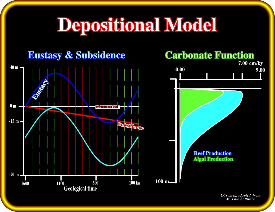
The Exxon carbonate depositional model is illustrated on Plate 313 using Marco Polo software. The parameters of eustasy and subsidence are exactly the same as those used in the sand-shale model (Plates 309 to 311). The relative sea level curve is the same in both models (Plate 312).
Plate 312- To build the carbonate sedimentary model shown in Plate 313, we have used the eustatic curve (in light blue) and the subsidence (in red) illustrated on the left. In the carbonate function (on the right), the algal and reef production are maximal (5-7 cm/ky) near the surface at 2-3 meters water depth. At around 70-80 meters of water depth, there is no more reef or algal production.
The only difference is the sedimentary input. In the previous sand-shale model, the sediments are transported from the continent toward the sea and the terrigeneous input is conventionally taken as constant (the surface between two consecutive chronostratigraphic lines is kept invariable). In the carbonate model, the sediments are created in place by algal and reef production. Such an organic production is a function of water depth. The maximum of production ranges between 2 and 3 m of water depth (Plate 312) and it decreases progressively towards the bottom of the photosynthesis zone. Below this limit (roughly 80-100 meters), the absence of light prevents all algal production. Actually, algal production disappears between 30 and 40 meters of water depth.
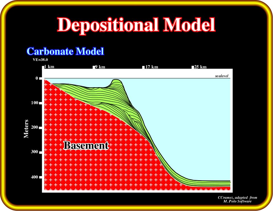
Plate 313- The sedimentary carbonate model illustrated here was built using Marco Polo software. The same relative sea level curve of the sand-shale model (Plate 330) was used here. Only, the terrigeneous influx was replaced by a carbonate function (Plate 312), in which algal and reef production are maximal near the surface (2-3m water depth). The unconformities as well as the different systems tracts composing the cycle sequences still are relatively easy to identify but their global geometry is quite different of the sans-shale cycle sequences.
Reef growth becomes nil at the compensation depth, i.e., at the lower boundary of the euphotic zone, which corresponds to the part of the ocean in which there is sufficient penetration of light to support photosynthesis.
(i) At first sight, the stratal patterns of the carbonate model look quite different from those associated with the sand-shale facies.
(ii) The geometrical relationships between the chronostratigraphic lines are the same.
(iii) Looking attentively, the same seismic surfaces, i.e., the surfaces defined by the reflection terminations are recognized, as well as the same systems tracts.
The same questions formulated previously for the sand-shale model are valid for the carbonate model, that is to say, explorationists using these models should not forget that:
1) Numerical models contain closed mathematical components that may be validated, just as an algorithm within a computer program may be validated ;
2) Finer scale structures and processes are lost from consideration, a loss that is inherent in a continuum mechanical approach ;
3) Exxon’ geologists assumed that the completeness of the stratigraphical interval deposited during a eustatic cycle of 3rd order was practically 100%. They assumed that the sedimentary processes were active during the entire time interval, i.e., sedimentation was a continuous process. Such an assumption is just not true. The completeness of a stratigraphic interval is seldom higher than 20%.
Sedimentary processes are discontinuous and catastrophic. In this perspective, one can say, Vail's sequence model is holistic. It forms a whole, in which the study of its parts (systems tracts) can only be approached when the organization of the whole is known. In other words, a sequence-cycle is a whole, composed by different parts, which by itself is, at the same time, a part of larger wholes, that is to say, continental encroachment sub-cycles and continental encroachment cycles.
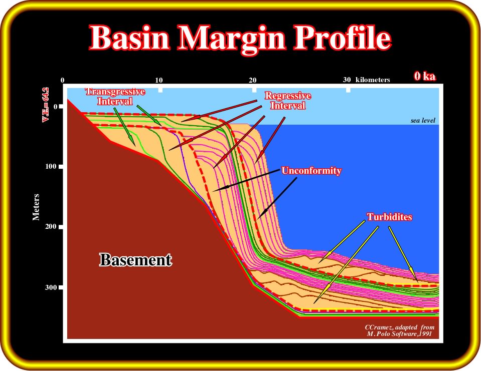
Plate 314 - The first thing a geoscientist must notice in this mathematical model is the vertical scale. In this particularly example, the vertical exaggeration is more or less 64 times, that is to say, far beyond the natural scale (1:1). Generally, the vertical exaggeration of the seismic lines ranges between 2 and 6 times. All models illustrated on the next plates are vertically exaggerated. Subsequently, the geometric relationships between defined by the chronostratigraphic lines are abnormally enhanced compared with those of the conventional seismic data.
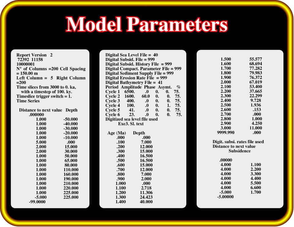
Plate 315 - This plate summarize the variables used in the models illustrated on next plates.
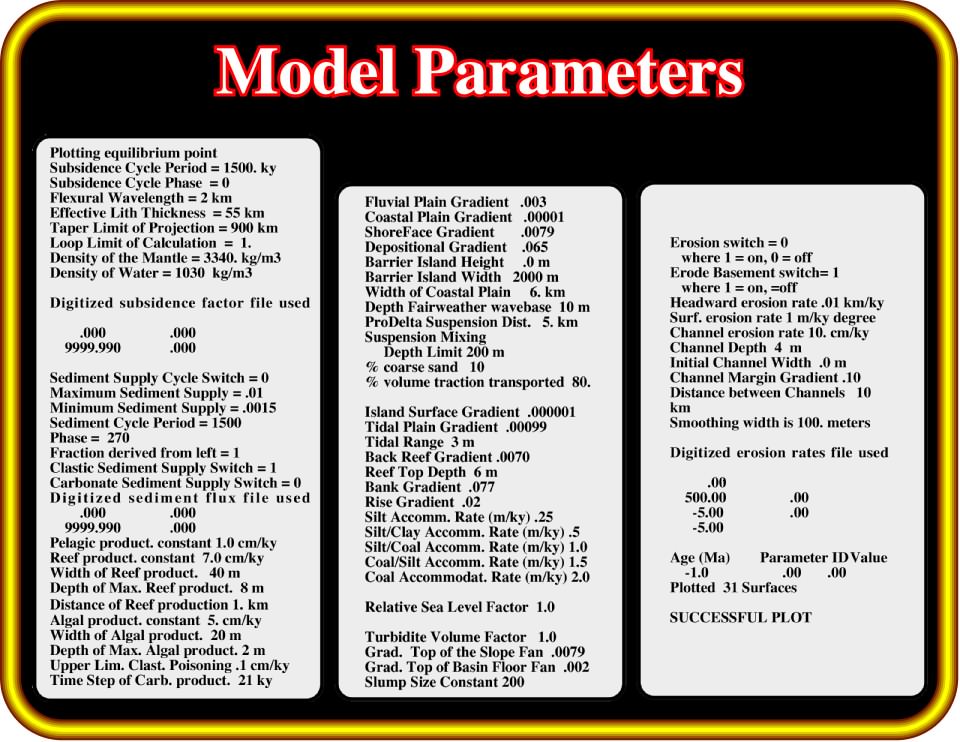
Plate 316 - This plate shows the others variables used in the models illustrated on following plates.
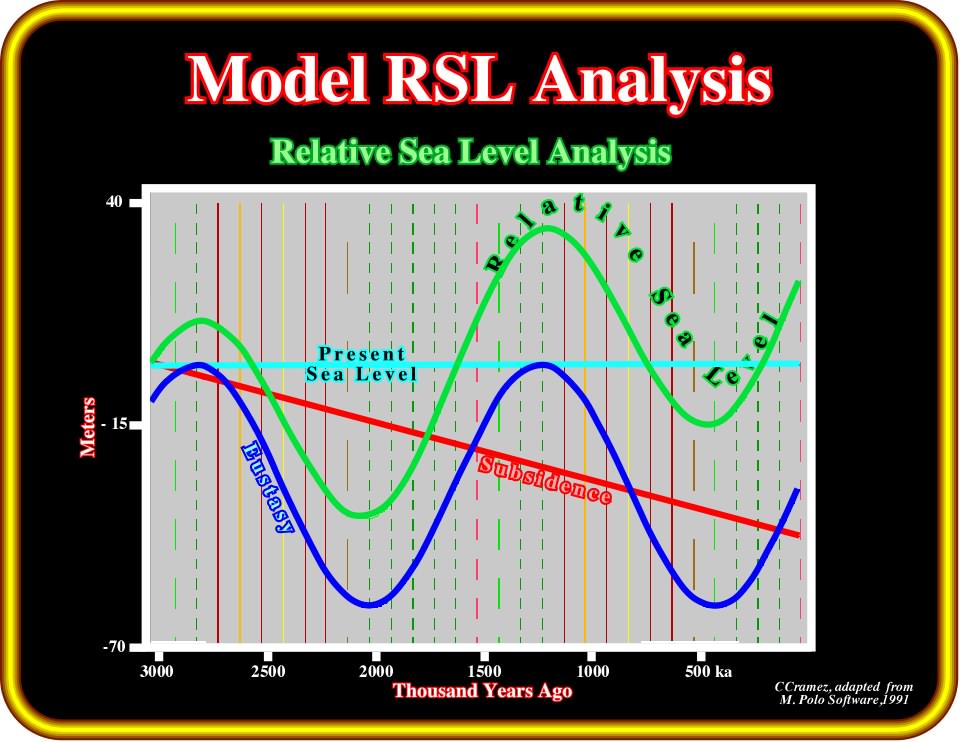
Plate 317- The subsidence (in red) combined with the eustasy (dark blue) gives the relative sea level, RSL, (in green), i.e., the space available for the sediments or accommodation, which controls the sedimentary evolution (between 3.0 Ma to 0 Ma). As illustrated, in this model, the accommodation increases from 3 Ma till 2.7 Ma., decreases from 2.7 Ma till 2.0 Ma., increases from 2.0 Ma till 1.3 Ma, decreases from 1.3 Ma till 0.4 Ma and finally increases till 0.0 Ma.
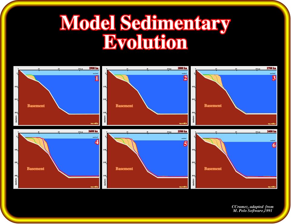
Plate 318- In this model, taking into account that (i) each step represents the sediments deposited during 100 ka, (ii) the terrigeneous influx (area between two consecutive chronostratigraphic lines) is constant and (iii) there is no erosion, one can say: (a) in step 1, a transgressive interval (transgressive systems tract, TST) was deposited ; (b) in steps 2 and 3, a relative sea level rise (RSLR) induced two regressive intervals (parasequences) forming a highstand systems tract (HST) ; (c) A relative sea level fall (RSLF) took place between steps 3 and 4, creating a type II unconformity and a shelf margin wedge (SMW) ; (d) the relative sea level fell during steps 4 and 5 creating an unconformity ; (e) a new sedimentary cycle (sequence-cycle) started in 6, with the deposition of the lower member of the lowstand systems tract (LST), that is to say a basin floor fan (BFF).
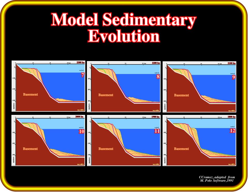
Plate 319- In the new sedimentary cycle (sequence cycle), overlying the basin floor fan (BFF), channel levee complexes of a slope fan (SF) were deposited during steps 7, 8 and 9. Then, since the relative sea level commenced to rise, the upper member of the lowstand systems tract (LST), that is to say, the lowstand prograding wedge (LPW) was deposit (step 10). During steps 11 and 12, relative sea level rose, and so, two new parasequence cycles were deposited in LPW.
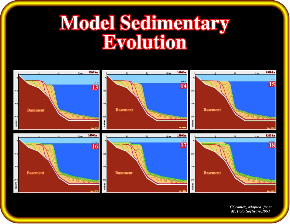
Plate 320 - During steps 13, 14 and 15, relative sea level rose and more parasequences of the lowstand prograding wedge (LPW) were deposited. Then, during step 16, the rate of relative sea level rise reaches its maximum, and so, the sea flooded the exhumed shelf inducing a transgressive systems tract (TST). In steps 17 and 16, the sea level rose, but in deceleration, so, a highstand systems tract (HST) started to deposit on the shelf, while in the deep parts of the basin starved conditions predominate.
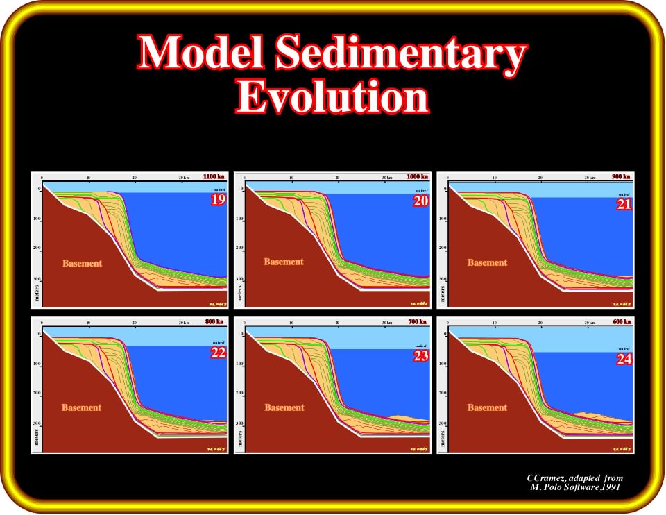
Plate 321 - In step 19, a small relative sea level fall created a type II unconformity and, in step 20, a shelf margin wedge (SMW) was deposited. In step 21, a relative sea level fall put the sea level below the coastal break, which was coincident with the shelf break (basin without shelf), creating a type I unconformity, which limits the sequence-cycle. At the same time (minimum hiatus), in the deep parts of the basin a new sequence-cycle started (step 22) with the deposition of a basin floor fan (BFF), i.e., the lower member of the lowstand systems tract (LST). In steps 22 and 23, channel-levee complexes, formed a slope fan (SF), deposited above the basin floor fan (BFF).
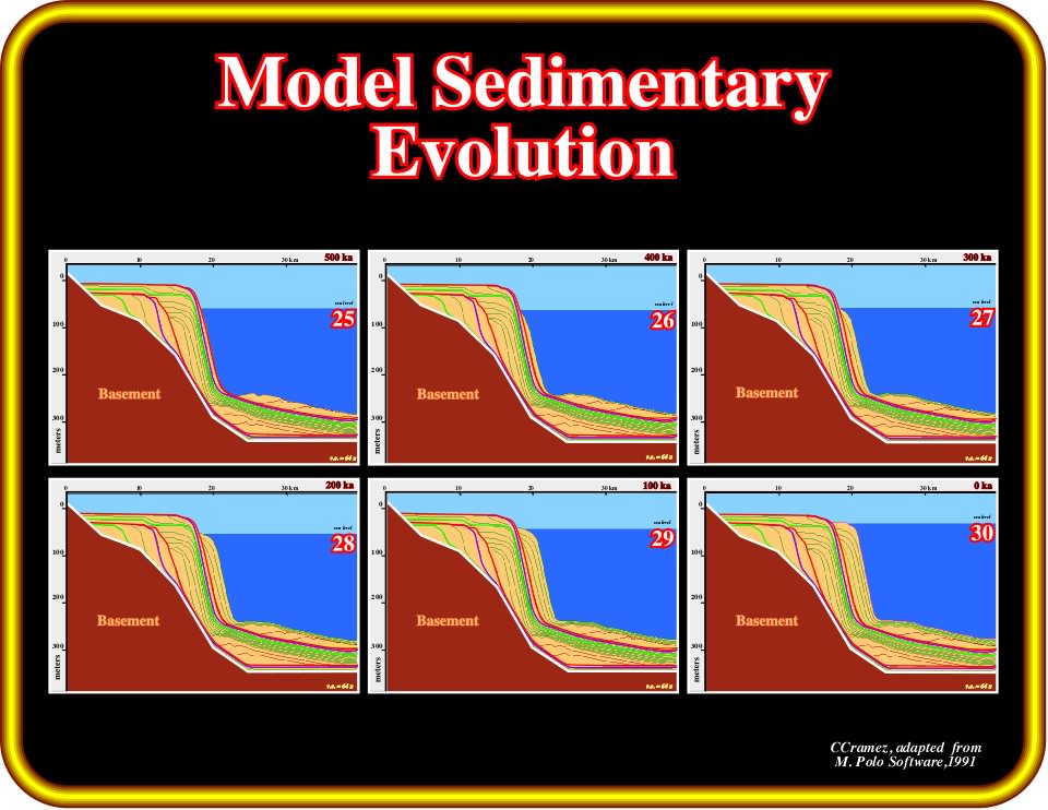
Plate 322- After the deposition of the uppermost channel-levee complexes of the slope fan (SF), in step 25, relative sea level started to rise, in acceleration, and so, the lowermost parasequences of the lowstand prograding wedge (LPW) commenced to deposit (step 26). Then, with the continuation of rise of relative sea level, during steps 27, 28, 29 and 30, the distal part of the LPW parasequences, progressively, fossilized, in downlap, the uppermost channel-levees of the slope fan.
to continue press![]()
![]()