C- Seismic Exploration Basic Review

- Basics Review

Seismic exploration is supported by the elastic wave propagation theory. The main relevant basic principles are:

a) Conservation of energy

b) Equations of motion (Newton’s laws)

c) Reciprocity

d) Linearity

Solutions of acoustical problems are quite simple in homogeneous and isotropic environments (Plate 26.21). However,   in most geological cases, such approximation is rough.

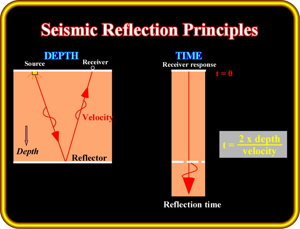
Plate 26.21- These sketches illustrate, in depth and time, the basic seismic mechanisms. The source, the depth of the reflector, the velocity of the sediments above the reflector, and the receiver are the main components of the seismic surveying. The time response is given by the depth of the reflector multiplied by the velocity of waves within the sediments overlying the reflector.

Theoretically, we can solve wave propagation equations and predict, if we know the movement of a particle at a point, the resultant movement at any other point. This is particularly true as long as we know the physical characteristics of the environment, especially the longitudinal velocity.

Seismic data acquisition (Plate 26.22) is designed to efficiently record, through surface receivers, energy from shot point after it is reflected off of subsurface elastic discontinuities.

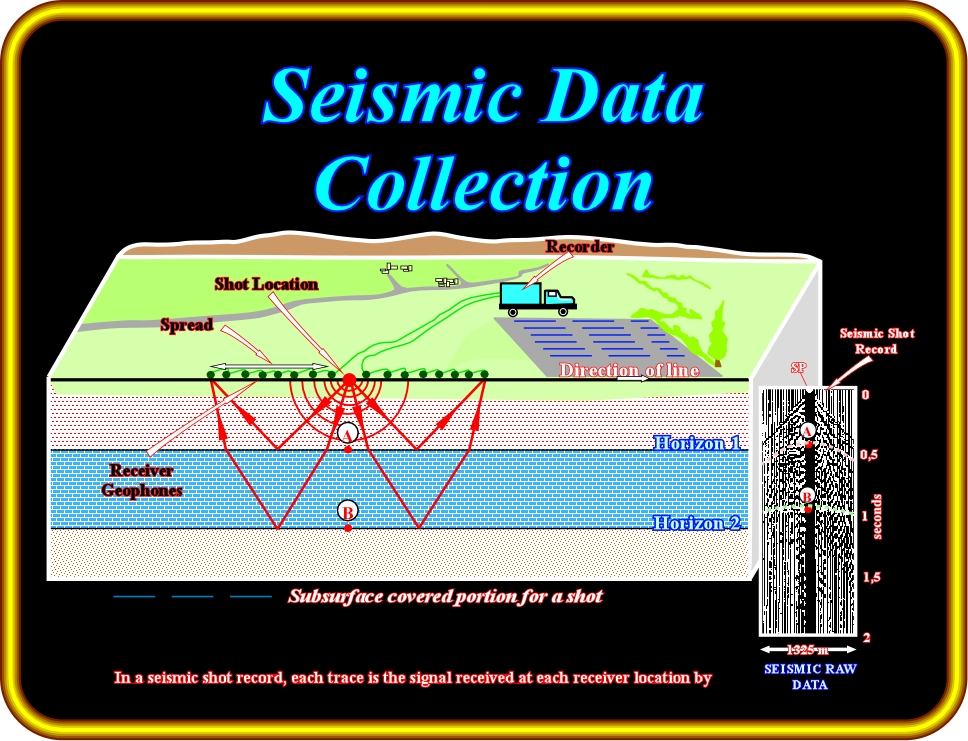
Plate 26.22- Acquisition and processing of seismic data require several steps. This cartoon illustrates land acquisition of seismic data. The source generates a low-frequency signal, which is reflected off an underground layer. A series of geophones picks up the arrivals of waves reflected at different angles to the source. The source and geophones are then moved, enabling every geophone to pick up reflections from various angles. These reflections are recorded on tape and the recordings displayed. Computer editing removes any noisy traces, and reflection signals from a common depth point are collected.

Conservation of energy (basic principle) implies that input energy must be either transmitted (surface wave, first arrivals), reflected, refracted, scattered (diffractions), converted into another wave type, or absorbed into heat. Conventionally, output energy is split in useful reflected energy or other forms of energy respectively called:

Signal and Noise

- Seismic Methods

Incident energy on an interface should be either (Plate 26.24):

- Reflected, i.e., the energy does not cross the interface (Plates 26.23, 26.24),

- Refracted, i.e. the energy travels along the interface, or

- Transmitted, when the energy crosses the interface.

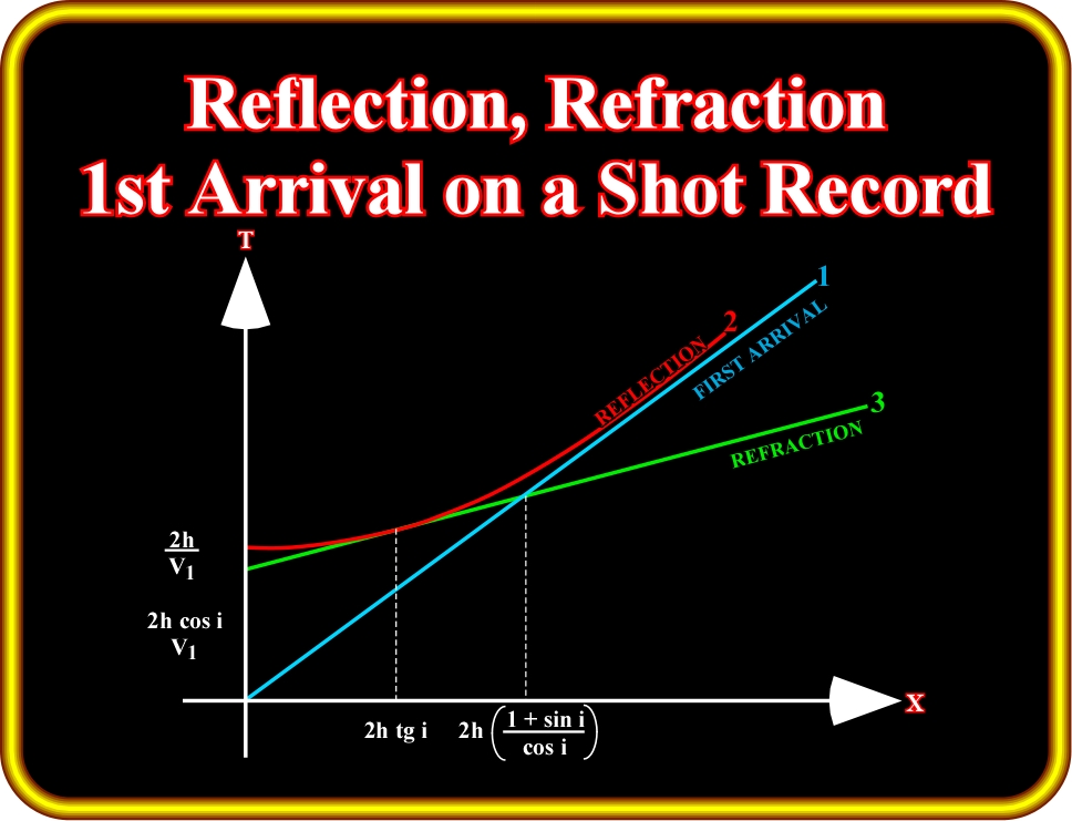
Plate 26.23- This figure illustrates the travel-time curves for direct (first arrival), reflected and refracted rays in the case of a simple two-layer model. The first arrival of seismic energy at a surface detector offset from a surface is always a direct ray or a refracted ray. The direct ray is overtaken by a refracted ray at the cross-distance 2h {(1+sin i)/cos i)}. Beyond this offset distance, the first arrival is always a refracted ray. Since critically refracted rays travel down to the interface at the critical angle there is a certain distance, know as the critical distance (2h tgi), within which refracted energy will not be returned to surface. At the critical distance, the travel times of reflected rays and refracted rays coincide because they follow effectively the same path. Reflected rays are never first arrivals. They are always preceded by direct rays and, beyond the critical distance, by refracted rays also.

Snell’s law controls all reflections within the critical angle, after which refraction occurs (Plate 26.24). The reflection is a function of the reflection coefficient, which corresponds to the ratio of the amplitude of the reflected wave to the incident wave (reflectivity). The ratio of the reflected energy to the incident energy is the square of reflection coefficient.

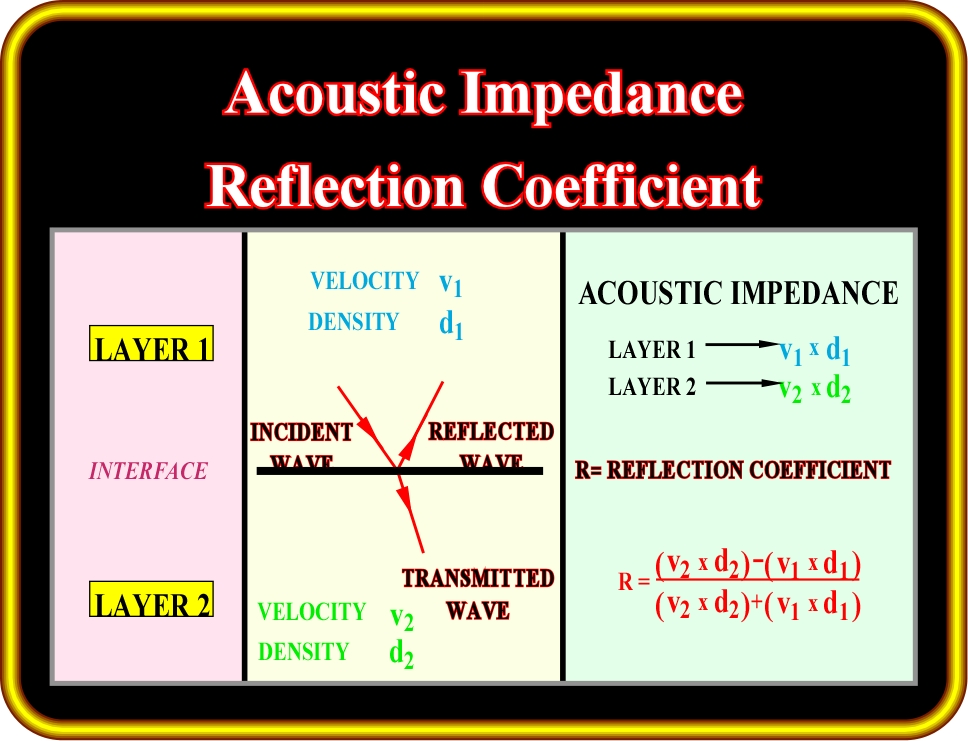
Plate 26.24- Assuming two sedimentary layers with different velocities (v1, v2) and different densities (d1, d2), i.e. with different acoustic impedances (v d), the reflection coefficient is the ratio between the difference of the acoustic impedance and the addition of the acoustic impedances. Notice that oblique incident waves on the interface are broken into reflected and refracted waves.

Depending on what we are looking for, we will have to select where to put receivers to pick either reflections or refractions for a given shot-point location and target. Refraction method was extensively used before the sixties. Unfortunately, today it is mainly limited to weathered zone bottom determination (small refraction).

D) Basics of Reflection Seismic

The basic principles of reflection seismic can be summarized in three steps:

(i) When a seismic wave is generated, the geophone picks up the wave‘s two way travel time down to a reflecting layer and back.

(ii) Moving the shot point and geophone generates a series of reflections of the layer.

(iii) Reflections show up as wiggly trace on the seismic record, which can be correlated across a profile.

In these notes, we assume that all explorationists are more or less familiar with the essentials of seismic prospecting, that is to say:

- Field work;

Spread, Source, Array, Digital Recording, etc.

- Processing;

Gain recovery, Filtering, Deconvolution, Velocity analysis, Stacking, Migration, etc.

- Signal Theory;

In waveforms of geophysical interest, the signal is almost invariably superimposed on unwanted noise. In favorable circumstances, the signal / noise ratio (SNR) is high, so the signal is readily identified and extracted for subsequent analysis. However, very often, the SNR is low and special processing is necessary to enhance the information content of waveforms. In order to make it clear, the aim of the geophysicist is:

- At acquisition stage:
To find the best compromise for penetration and resolution of the data according to the exploration target.

- At processing stage:
To extract the maximum benefit of recorded data in terms of reliability, geometrical control, and definition.

- At interpretation stage:
To organize observations through an understanding and acceptable a priori geological model. In other words, interpreters start always with a geological problem. In order to solve it, they propose a hypothesis, which they try to falsify. If the refutation test is positive, they get a new problem, which obliges them to propose a new hypothesis ...., a new test ..... and so on. This scientific method is often called pragmatic, rational or hypothetico-deductive.

Seismic Reflections

The sound waves travel in all directions, but only those traveling almost directly downward can be reflected off structures (interfaces) underneath the explosion. A seismic reflection (Plate 26.25) is produced at any break of acoustic impedance (product of the seismic velocity and bulk density).

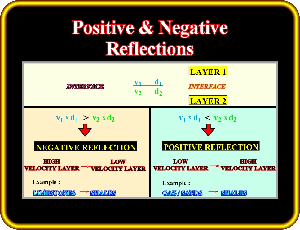
Plate 26.25- A negative reflection occurs when the acoustic impedance of the upper layer of the interface is higher than that of the lower layer (ex: limestone / shale, or shale /sandstone). When the acoustical impedance of the lower layer is higher than that of upper layer the associated reflection is positive (ex: shale /limestone, etc.).

Seismic reflections can be positive or negative and their polarity can be to the right or to the left (Plates 26.25 and 26.26). Seismic waves are modified by acoustic impedance discontinuities in forms of changes of amplitude and polarity.

Plate 26.26- The SEG polarity convention assumes that for a positive reflection coefficient (low acoustical impedance / high acoustical impedance) the amplitude is expressed by a deflection to the right of the base line (black) and to the left (white) for a negative polarity.

In general terms the amplitude for a symmetrical waveform is half of the orthogonal distance between the crest, or ripple, above the adjacent troughs (for asymmetrical and non-periodic systems, other definitions have been proposed).

As seismic waves arrive at the Earth’s surface, the amplitude of a seismic signal decreases rapidly with time. This amplitude range is very large, often a million to one or more:

- The eye can appreciate this range, from 1mm to 1 km, but it is clearly quite impractical to present the results in this range.

- On standard cross-sections, the eye does not appreciate anything much outside a 10 to 1 range in amplitude, that is to say, amplitudes from 0.1 mm to 1mm.

- Amplitudes must be constrained within this range, either by automatic (data dependent) processes or purely functional changes.

- Data Acquisition

1- In onshore

On land the returning sound wave is detected by a listening device called a geophone. A single shot recorded by a single geophone is recorded on a strip chart as a long line, with a pulse representing the time when the reflected sound wave returned. If more than one reflecting surface is encountered, there will be more than one pulse on the trace. The vertical scale on most seismic lines is therefore two-way travel time (t.w.t.) in seconds.

Knowledge of the average seismic velocity of various rock types enables interpreters to calculate the actual depth of reflecting layer in meters rather than in seconds, but this is needed only when they are trying to match seismic records with electrical logs or surface outcrop. A single strip chart is as one-dimensional as a borehole record. To get two-dimensional layers and other structures, an array of recording points is needed.

Every point records the shot separately and produces a strip chart. When all the charts are lined up, the pulses, or reflections from the same layer also line up from one chart to the next, and the first approximated measurement of the layer is made. This is called picking the marker reflections.

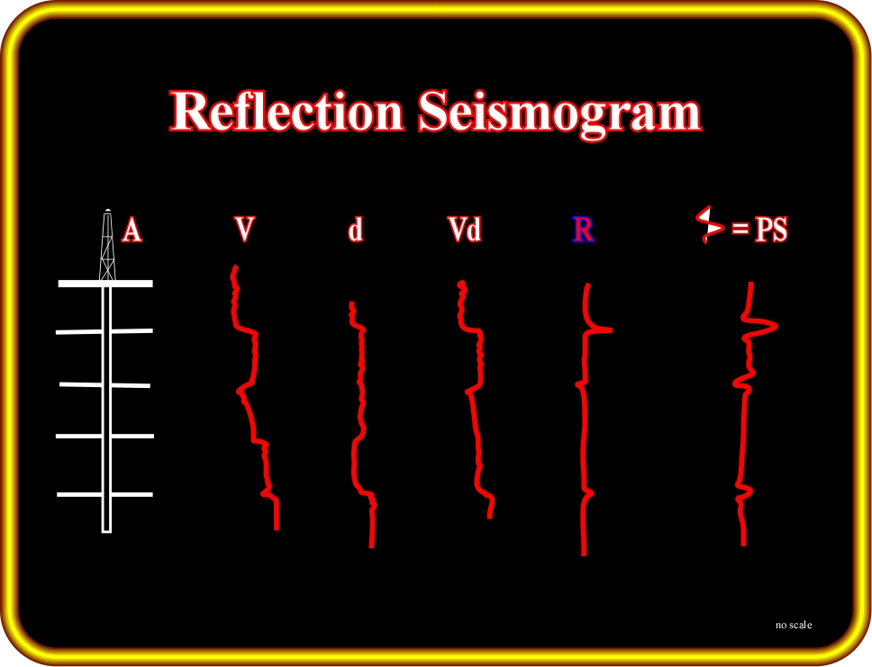
Plate 26.27- The reflection seismogram can be seen as the convoluted output of a reflective function with an input pulse. Assuming the pulse shape remains unchanged as it propagates through such a layered ground, the resultant seismic trace may be regarded as the convolution of the input pulse with a time series known as a reflectivity function (R). The amplitude of each spike is related to the reflection coefficient of a boundary and a travel time equivalent to the two-way reflection time for that boundary. This time series represents the impulse response of the layered ground. V represents the velocity of the seismic waves in the sedimentary intervals drilled by the well A, d represents the density of the sedimentary intervals, Vd is the impedance profile and R is the reflectivity function. PS is the pulse shape.

The geophones in an array are laid out in a traverse at regular intervals away from each record truck, which contains the instruments to record the signals and the computer to process and interpret them. The sound is then generated using dynamites or vibrators. Every geophone in the line array picks up the direct reflection at a time that depends on the distance between the acoustic source and the reflector.

The earth motion, which the geophysicist sets out to record, consists of the wanted and unwanted parts of the earth response to the input. Some of the sources of unwanted signals/noise are:

- Earth is a noisy place.

- There are many other seismic and acoustic sources in operation at any time.

- The sources that are very close to the detectors produce signals, which appear quite random. Ex: Grasshoppers on the geophones.

- Arrival from more distant sources may be recognizable on many detectors.

- Distant sources generating periodic waveforms, such as ships, trains, airplanes, power stations and other industrial processes, will add rather similar wave-forms to all the data.

The skills of seismic data gathering are directed to reducing the noise content in the recorded signal, and data processing to improving still further the signal-to-noise ratio.

To improve the signal-to-noise ratio after a shot is made, the source and its array are moved a distance down-line, so that the reflections from the same layer will be picked up by geophones from slightly different positions. This is called the common-depth-point method.

By repeating the shots and measuring from slightly different positions along a linear transect, the signals are recorded many times and can be stacked or summed together. This amplifies the signals and screens out the noise because the noise has no regular pattern along the line. Finally, all the signals from the single traverse are collected, screened by the computer, and printed out as a seismic profile.

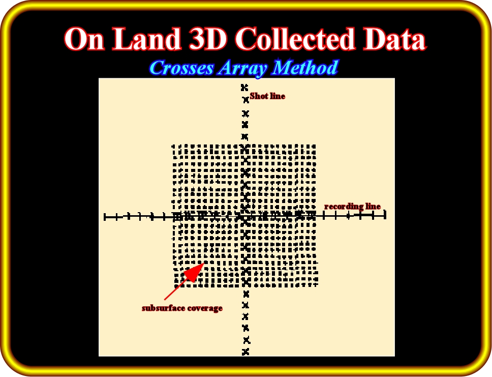
Plate 26.28- On land, three dimensional data are normally collected using the cross array method, in which shots and detectors are distributed along orthogonal sets of lines (in-lines and cross-lines) to establish a grid of recording points. This sketch illustrates for a single pair of lines, the area coverage of a subsurface reflector.

It should be noticed that if most of seismic reflections are associated with chronostratigraphic horizons or stratification planes, it is possible that significant geological interfaces are not captured as seismic reflectors. That happens when there is no impedance break associated with the interface:

V1 x d1=V2 x d2

2- In offshore

The basic method of acquiring seismic data offshore is much the same as that of onshore, but it is simpler, faster and hence cheaper. A seismic boat replaces a truck as the controller and recorder of the survey. This boat trails an energy source and a cable of hydrophones, termed a streamer (Plate 26.29).

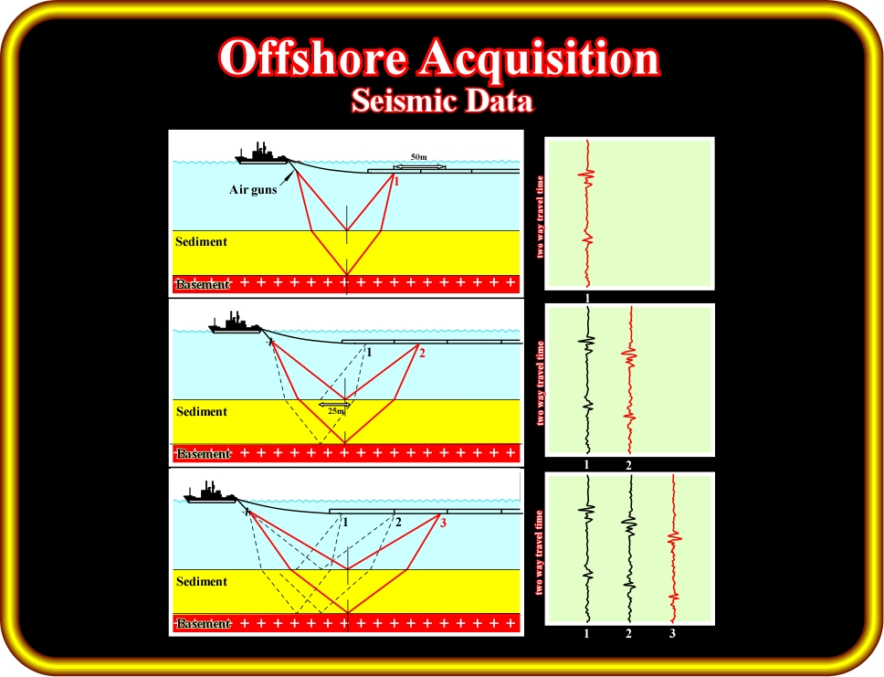
Plate 26.29 - Example of offshore seismic data collection (three traces).

It is possible for one boat to operate several energy sources, but experience has shown that more bangs is not necessarily best.

- Streamer lengths can extend for up to more than 8000 m to the annoyance of fisher folks.

- Currently, surveys vessels can operate up to three energy sources whose signals are received by hydrophones on 8 to 12 streamers, up to 3000 m in length, with a total survey width of 800 m.

- In marine surveys, dynamite is seldom used as an energy source:

a) For shallow high-resolution surveys, including sparker and transducer surveys, high frequency waves are used.

b) For deep exploration, the air gun is widely used as the energy source.

In the air gun method, a bubble of compressed air is discharged into the sea. Usually a number of energy pulses are triggered simultaneously from air guns:

- The air guns emit energy sufficient to generate signals more than 10 seconds two-way-time.

- Depending on interval velocities, these signals may penetrate to more than 5 km.

The reflected signals are recorded by hydrophones on a cable towed behind the ship. The cable runs several meters below sea level and may be more than 8 km in length. As with land surveys the CDP method is employed and many recorders may be used.

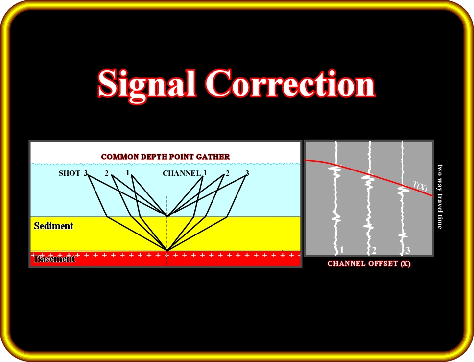
Plate 26.30 - The signal correction attempts to eliminate the time differences between reflection times, resulting from changes in the outgoing signal from shot to shot.

The reflected signals are transmitted electronically from groups of hydrophones along the cable to the recording unit on the survey ship. Other vital equipment on the ship includes a fathometer and position fixing devices:

- The accurate location of the shot points at sea is obviously far more difficult than it is on land.

- Formerly, this was done either by radio positioning, or by getting fixes on two or more navigation beacon transmitters from the shore.

- Nowadays, satellite navigation systems enable pinpoint accuracy to be achieved.

The steps in signal reprocessing are:

(i) - Gathering

(ii) - Offset

(iii) - Enhancement

(iv) - Stack

(v) - Addition

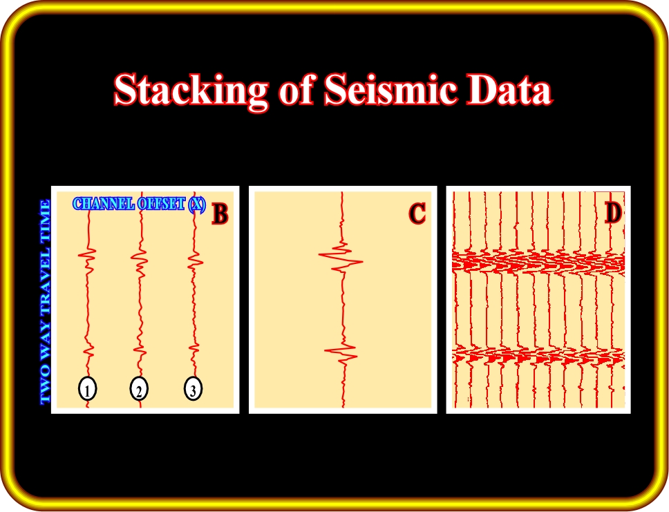
Plate 26.31 - Since the recording reflections are gathered from a CDP, the traces are shifted so that corresponding peaks have the same arrival time. Then, the traces are added and the reflection peaks are enhanced. Finally, thousands of point profiles are put side by side and the peaks area darkened according to the SEG convention.

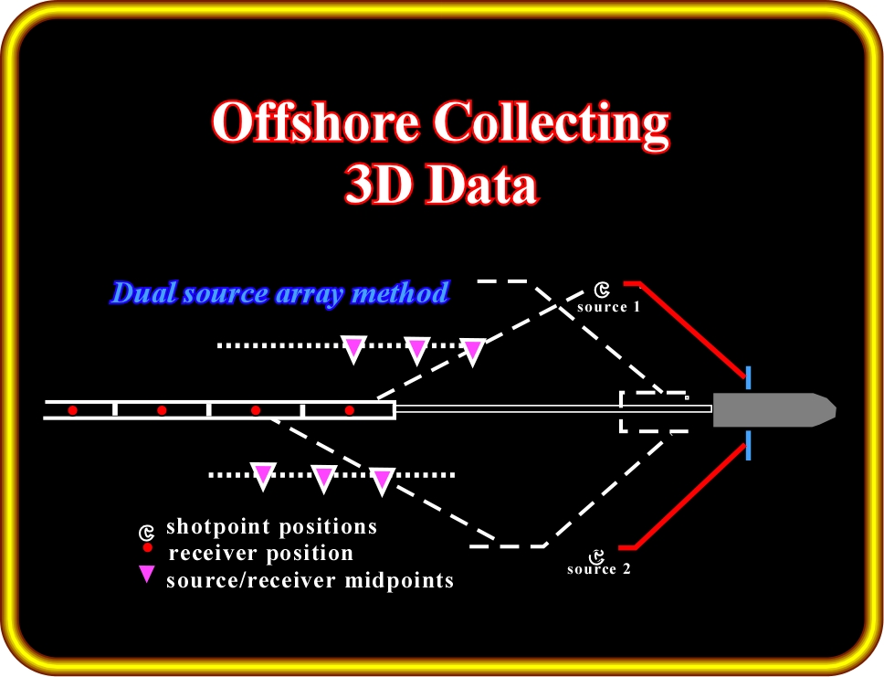
At sea, three-dimensional data may be collected along closely-spaced parallel tracks with the hydrophone streamer feathered to tow obliquely to the ship‘s track such that it sweeps across a swathe of the sea floor as the vessel proceeds along its track. By ensuring that the swathes associated with adjacent tracks overlap, data may be assembled to provide the coverage of subsurface reflectors.

Plate 26.32 - This cartoon illustrates the dual source array method of collecting three-dimensional seismic data at sea. Alternative firing of sources 1 and 2 into the hydrophones produces two parallel sets of source detector midpoints.

In the alternative dual source array method, sources are deployed on side gantries to port and starboard of hydrophone streamer and fired alternatively (Plate 26.32). Dual streamers may similarly be deployed to obtain three-dimensional data.

High quality position fixing is a prerequisite of three-dimensional marine surveys to ensure that the locations of all shot-detector midpoints are accurately determined.

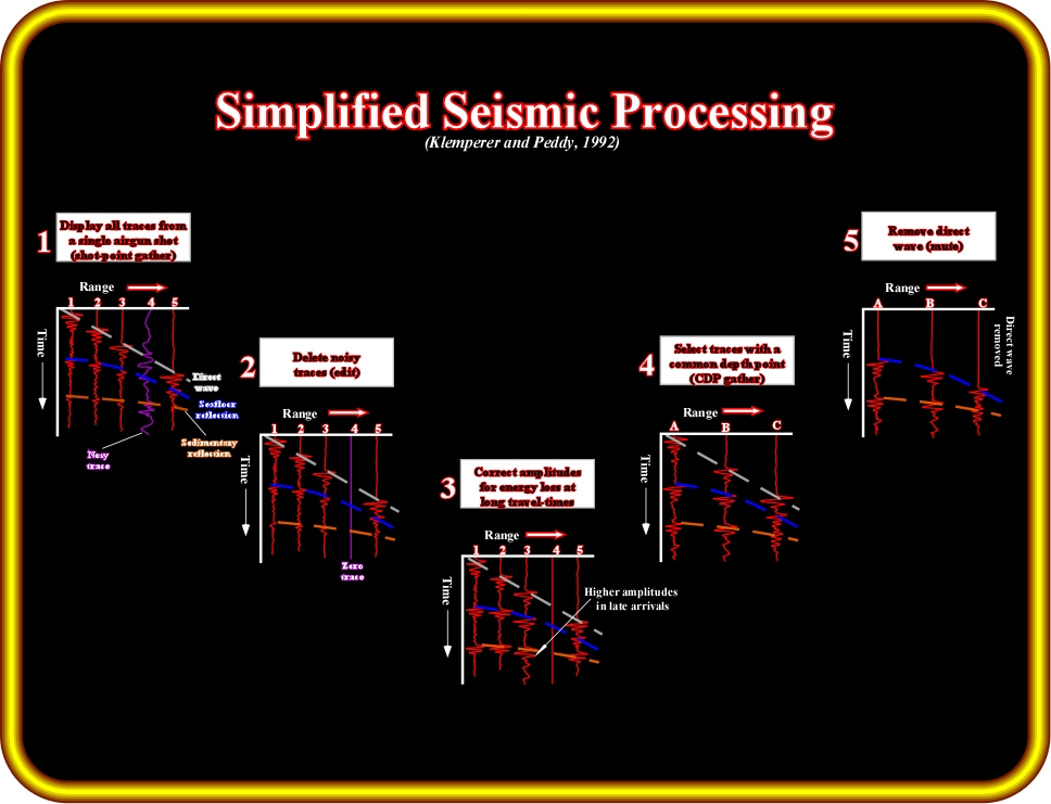
Plate 26.33 - The traces illustrated in part (1) result from a single shot, and were recorded by a single receiver. The direct wave (refracted wave) appears at a time proportional to the receiver distance from the shot, while the reflections lie on a hyperbolic travel-time curve. Any bad or noisy traces are deleted (2). The seismic amplitudes recorded decrease with increasing travel-time because the reflectors are further away, so the weaker amplitudes are boosted (3). Then the traces are resorted so that all traces with an identical source-receiver midpoint are gathered together in (4), one trace each from (1), (2), and (3). The direct wave is removed (the shaded area in 5). (see next Plate).

Position fixing is normally achieved in near shore areas using radio navigation systems, in which a location is determined by calculation of range from onshore radio transmitters. Beyond the range of such systems satellites navigation is used, with Doppler sonar being employed to determine the velocity of the vessel along the survey track for interpolation of position during the time interval between individual satellites fixes.

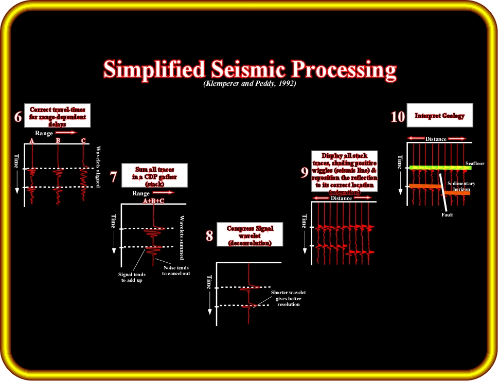
Plate 26.34 - Each trace is separately corrected for the time-delay appropriate for its source-receiver offset (6). This is known as the normal move-out, or NMO correction. The wavelets from each reflection are now lined up, as if each trace had been recorded with coincident source and receiver (i.e., without source-receiver offset delays), and all the traces in the gather can be summed (stacked) to give a single trace in (7) with a higher signal-to-noise ratio. If the wavelet is rather reverbatory, or lengthy, then its resolution is poor, but can be shortened by a digital filtering technique called deconvolution (8). Finally, all the traces are displayed as a seismic section and may then be interpreted (Selley, 1998).

to continue press