
Another common difficulty encountered in the seismic interpretation is the presence of some organized energy not originated by reflectors in the vertical plane defined by the profile, i.e., lateral arrivals. These conditions may defeat the interpreter if he attempts to interpret a seismic line in isolation, in other words, geoscientists should avoid to propose geological tentatives interpretations based just in one seismic line. Each system of reflections may show sections of continuity, with areas of confusion between them. Without further evidence one cannot tell which continuous reflections are related to which others, nor can one tell the directions from which they arrive. Sometimes, the examination of other lines with better orientations, will reveal enough of the structure to enable one to interpret these complex sections with arrivals from various directions (“side-swiper”).
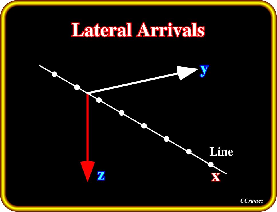
Plate 50- Lateral arrivals, that is to say, the presence of organized energy not originated by reflectors in the vertical plane Z defined by the profile, arequite common in seismic lines, particularly in 2D data. As depicted here, the lateral arrivals can arrive from any direction. In fact, the angle entre x (profile) and y (energy source) can be 0 or 90°.
One of the interpretation hazards that a seismic migration attempts to resolve by re-establishing true dips, is the one created by reflections generated off the plane of the section. Dips are not always perpendicular to the vertical plane determined by the field layout of the recording spread. If lateral dip component, relative to this plane, exists, some of the recorded events at least will be generated from areas that are off the vertical plane of the section. Only tri-dimensional seismic data, processed through 3D migration, can accurately place all reflections to their true location space.
Example:
The seismic line illustrated in Plate 51 shows a misleading well marked lateral arrival, which was initially interpreted by some geoscientists as the trace of a reverse fault. They recognized two faulted blocks with an important shortening on the up-thrown block and they associated the diachronic reflector with a fault plane. However, such an association is rarely observed. Generally, on a seismic lines, fault planes are recognized by the associated seismic surfaces, that is to say, loci of reflections terminations and not by reflectors.
However, few exceptions are well know. Seismic reflectors can be recognized with:
(i) Fault planes intruded by volcanic or evaporitic material ;
(ii) Well developed gouge zones ;
(iii) Strong impedance contrast between fault blocks ;
(iv) Fault planes between sediments and basement, etc.
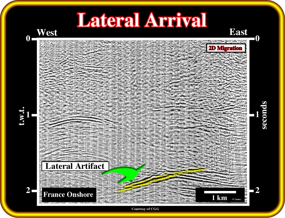
Plate 51- The reflector (yellow) indicated by the green arrow was initially interpreted as the trace of a reverse fault plane developped to acommodate the shortening of the sediments. However, in spite of the fact that such interpretation is compatible with the regional geological setting, there is no logical reason (impedance contrast) to have a reflector underlying the fault plane. Actually, it seems to correspond to a lateral seismic artifact. The 3D data, illustrated on Plate 52, corroborates the lateral artifact conjecture.
The same seismic profile was rebuilt using 3D data (random line, Plate 52). It clearly indicates there is any oblique diachronic reflector on the vertical plane defined by the profile. Such an absence corroborates the hypothesis that the oblique reflector, recognized on the 2D data (Plate 51), corresponds to a lateral arrival.
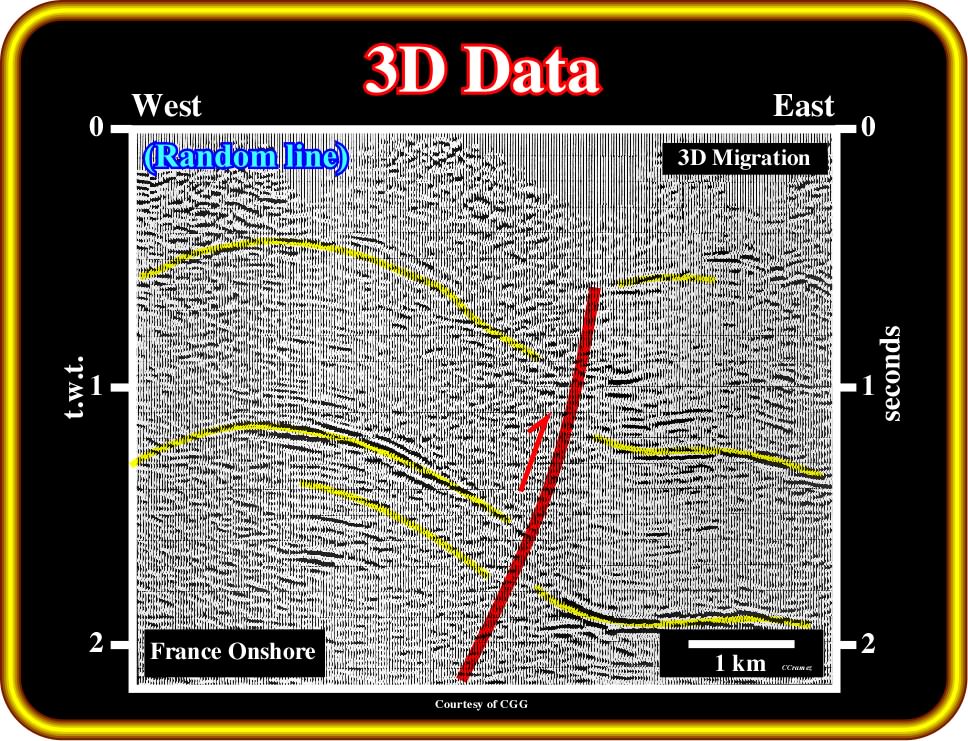
Plate 52- The 3D random seismic line along the trace of the previous line corroborates the hypothesis that the oblique diachronic reflector on Plate 66 corresponds to a lateral arrival (sidewinder). Nevertheless, geologically speaking, this seismic line illustrates a faulted compressional structure, in which a reverse fault plane can be recognized by a seismic surface defined by reflection terminations. As we see later, in the majority of the cases ( there are few exceptions), there are no seismic markers highligthing the fault planes.
The essential difference between two-dimensional and three-dimensional migration may be illustrated with reference to a point reflector embedded in an homogeneous medium. On a seismic section, derived from a two-dimensional survey, the point reflector is imaged as a diffraction hyperbolae and migration involves summing amplitudes along the hyperbolic curve and plotting the resultant event at the apex of hyperbolae.
The actual three-dimensional pattern associated with a point reflector is a hyperbolic of rotation. Diffraction hyperbola recorded in a two-dimensional survey represent a vertical slice through this hyperbolic. In a 3D survey, reflections are recorded from a surface area of the hyperbolic and three-dimensional migration involves summing amplitudes over the surface area defining the apex of the hyperbolic. A practical way of achieving this aim with crossed-array data, from a 3D land survey, is the two-pass method:
- First pass involves collapsing diffraction hyperbolas recorded in vertical sections along one of the orthogonal line directions ;
- Series of local apexes, in these sections, together define a hyperbola in a vertical section along the perpendicular direction ;
- Hyperbola can then be collapsed to define the apex of the hyperbolic.
So far, we have examined velocity anomalies and dip related distortions. In either case, recorded events, though displaced from their true position, image somehow a reflecting horizon and have therefore geological significance. Now, we will consider a different set of seismic events, which, though recorded as data, bear no relationship whatsoever to geology.
to continue press
![]()