
Universidade Fernando Pessoa
Porto, Portugal
Seismic-Sequential Stratigraphy
A shale dome‘s geometry (Plate 104) induces important lateral and vertical changes in velocity intervals. Due to diapirism, low velocity sediments will be pushed-up and juxtaposed to higher or lower velocity sediments. So, a planar bottom of a shaly facies, either horizontal or tilted on time seismic, generally has a pull-down geometry (Plate 104).
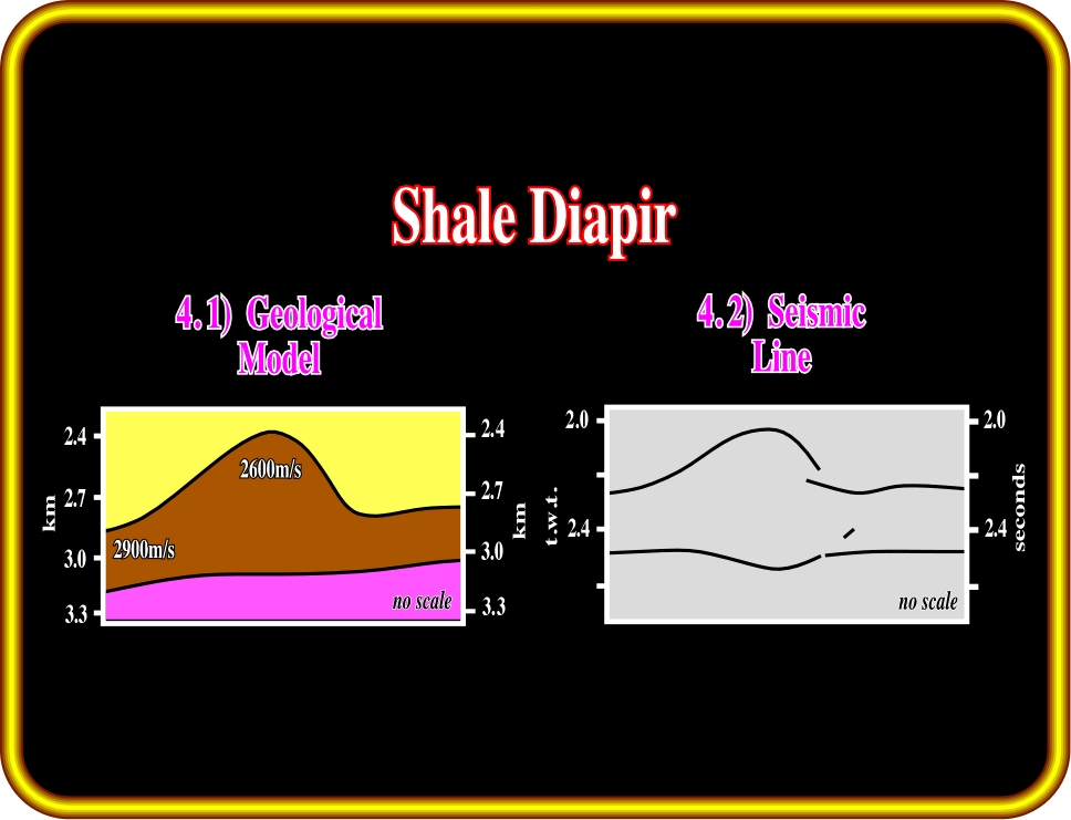
Plate 104- On this figure are illustrated a geological model of a shale mound and the equivalent seismic line. In the geological model, the shale interval (brown) has velocities ranging between 2600 and 2900 m/s.
In the majority of the cases, unfortunately, it is very difficult to see the root of the shale domes. Similarly, on unmigrated lines, due to the complex geometry of the reflections associated with the top of the shale, only the uppermost part, that is to say, the apex of the reflection associated with the domes, is in its real time position. In certain evaporitic basins, salt and shale domes can be present with similar geometries. One of the best ways to differentiate them is to look at the seismic markers emphasizing their bottoms. As stated previously, generally, the base of a shale dome has a pull-down geometry, while the bottom of salt dome shows a pull-up geometry. However, the bottom of salt domes are easier to recognize.
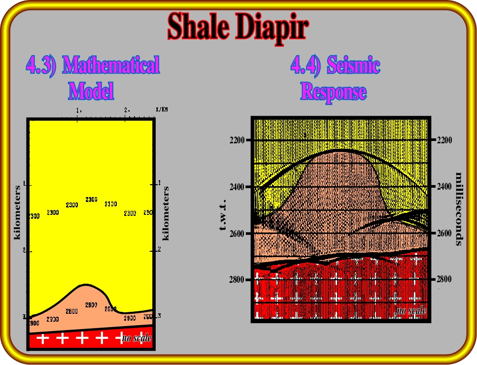
Plate 105- In the velocity model, the yellow sediments above the shale mound have a constant velocity of 2300 m/s. The velocity in the shale interval is 2600 m/s in the upper part, and 2900 m/s in the lower part. The seismic response of such a mathematical model indicates that the velocity contrasts are not big enough to significantly pull-down the bottom of the shale interval directly below the apex the vertical of the mound. Notice the seismic response is unmigrated, so only the apex of the mound is in its real position.
An interpreted seismic line of a salt dome and the correlative depth conversion (Plate 106) clearly illustrates the seismic anomalies associated with salt thickness variations.
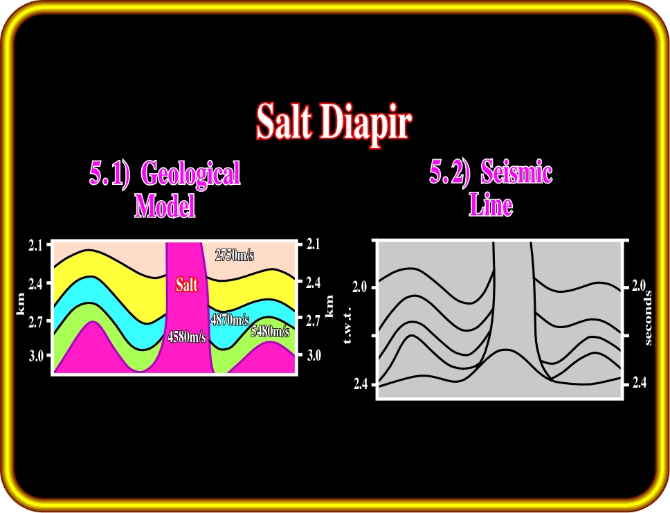
Plate 106- In the geological model, the compressional wave velocity of the salt is constant and equal to 4580 m/s. The density of the salt ranges between 2.15 and 2.17 g/cm3. In addition, salt cannot be compacted, that is to say, its density is constant and so its velocity does not change in depth. The velocity interval of the suprasalt strata is supposed to be laterally constant. On the seismic line of such a geological model, illustrated on the right, the bottom of the salt layer is undulated. It is pulled-up under the thick salt.
In this particular example the salt interval, which has a velocity of 4580 m/s, is overlain by sediment with calcareous facies that has a high compressional wave velocity (around 5480-4870 m/s). So, when the salt flows laterally, is locally thinner, hence, the result is a pull-down of the reflectors (salt velocity is relatively slower than the limestones velocity). On the contrary, when there is an upward movement of the salt, it is juxtaposed to sediments with a lower compressional wave velocity and the final result is a pull-up of the reflector associated with the bottom of the salt. In other words, when a salt layer is not isopachous, the bottom of the salt is pulled-up at under the thick salt zones and pulled-down where the salt is thin or not present (salt weld).
A velocity model and its correlative seismic answer (Plate 107), clearly illustrate the causes of apparent wavy geometries on the bottom of evaporitic packages on time lines (unmigrated or not).
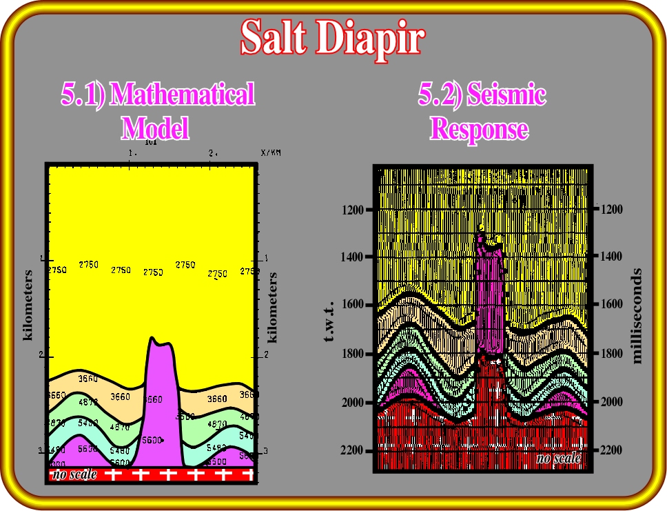
Plate 107- The seismic response to the geological model is quite evident. The bottom of the salt, particularly under the apex of the salt dome, is pulled-up almost 0.2 seconds (t.w.t.). Similarly, the salt welds (absence of salt due to lateral and vertical flowage) are slightly pulled-down. Note that this geological model of a salt dome with vertical flanks is unrealistic. Actually, due to the fact that salt cannot be compacted, salt structures with vertical flanks are physical impossibilities.
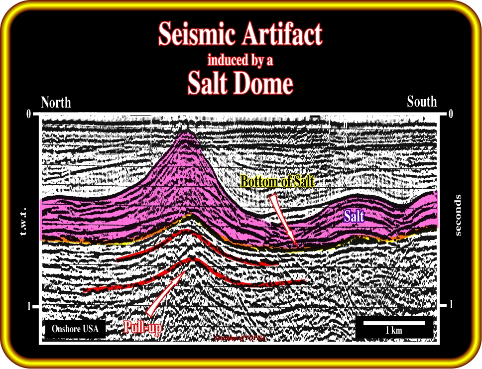
Plate 108- This seismic line from onshore Louisiana illustrates a seismic artifact induced by an evaporitic interval. The bottom of the salt layer is pulled-up where the salt interval is thicker.
The above seismic comes from an evaporitic basin where lateral changes in salt thickness are frequent. These thickness changes induce lateral changes in the velocity interval, which cause obvious seismic artifacts. However, without a corrected time-depth conversion, it is sometimes dangerous to assume, a priori, a flat salt bottom. Indeed, it has been shown, for instance in offshore Angola, that salt steps are often observed in association with major fracture zones.
The development of reefs or organic build-ups in which the seismic waves often have a high velocity, induce important pull-ups of the horizons associated with their bottoms, as is sketch in Plate 109. Nevertheless, generally, on the ground, hence, in geological models, reefs have bottoms showing planar geometries. A seismic line of such a reef is sketched below.
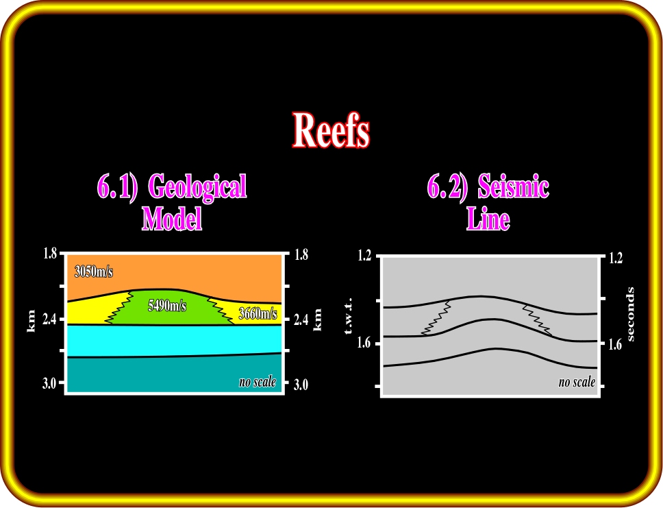
Plate 109- On this reef geological model, above a planar limestone sole (light blue), a reef with a compressional wave velocity of 5490 m/s, is laterally bounded by shaly sediments (yellow) with a much lower velocity (3660 m/s), which are overlain by even slower sediments (brown interval, 3050 m/s). The seismic answer of such a model is roughly depicted on the right. The horizon associated with the bottom of the reef shows a significant pull-up.
This geometry, with a pull-up of the bottom of the reef, is normal when the reef is developed adjacent to a low velocity interval such as shale. However, if a porous reef is developed within a tight calcareous environment, the geometry of the bottom of the reef is inverted, that is to say, the associated marker, if there is a marker, is pulled-down. Actually, in certain basins, for instance in the Michigan basin (USA), the recognition of reefal anomalies is mainly based in the absence of reflector. In other words, when, in a continuous and high amplitude marker, emphasizing a limestone interval, an abrupt interruption of the reflector occurs during few kilometers, it may be due to the presence of a local porous reef.
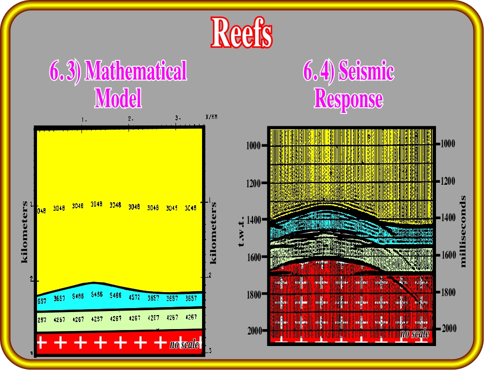
Plate 110- Notice that in the geological model the compressional wave velocity, in the blue interval (limestone with a local reefal development) changes significantly. It is much higher (around 5500 m/s) in the reef than in the surrounding sediments. Such a reef is supposed to be tight. The seismic response of such a model, on the right part of the figure shows that not only the bottom of the reef, but all others markers below are pulled-up.
The pull-up of the bottom of the reef is very sharp, as is the time thickness interval of limestone facies, which is clearly thicker in the velocity model. As said previously (Ashstart field, in offshore Tunisia) this kind of seismic artifact occurs very often near the platform limit-upper slope, where shelf margin reefs build-up, particularly in regressive stratigraphic intervals. The next figure (Plate 111) illustrates an instance taken from offshore Indonesia.
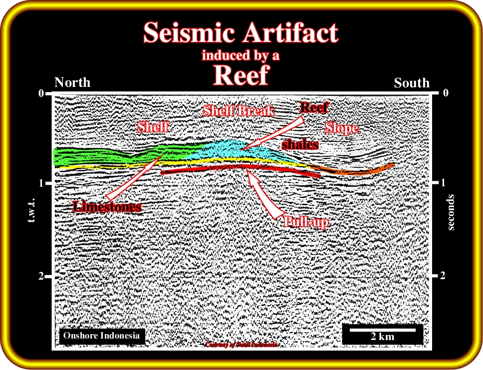
Plate 111- On this seismic line, from offshore Indonesia, the shelf break of the upper colored interval seems to emphasize the development of a reef. Actually, the bottom of the shelf limestone is pulled-up. This pull-up is enhanced by the pull-down of the reflectors associated with the slope shales (in brown).
to continue press
![]()