Universidade Fernando Pessoa
Porto, Portugal
Seismic-Sequential Stratigraphy
This method is based on measurements of small variations in the magnetic field:
- Indeed, as most sedimentary rocks are nearly non-magnetic, all inhomogeneous composition of basement rocks, or important topographic relief of the basement surface cause variations in the magnetic field.
- These variations can be measured by sensitive magnetometers at surface or, more commonly, by suitable instruments carried in an aircraft or behind a ship.
The measured variations in the magnetic field are interpreted in terms of the probable distribution of magnetic material below the surface, which in turn is the basis for inferences about the probable geological conditions (Plate 7).
Negative anomalies occur on the north sides of the buried magnetic masses in the northern hemisphere, and on the south side in the southern hemisphere. Maximum anomaly occurs at the poles and minimum anomaly at the equator.
The most important results of magnetic interpretation are:
(i) Depth determination of the basement rocks, or the thickness of sediments, and
(ii) Determination of local paleo-highs of the basement surface.
The interpretation of magnetic anomalies is similar, in its procedures and limitations, to gravity interpretation as both techniques utilize natural potential fields based on inverse square laws of attraction. The force F between two magnetic poles strengths m1 and m2 separated by a distance r is given by:
F =
m1m2 /4
r2
where,
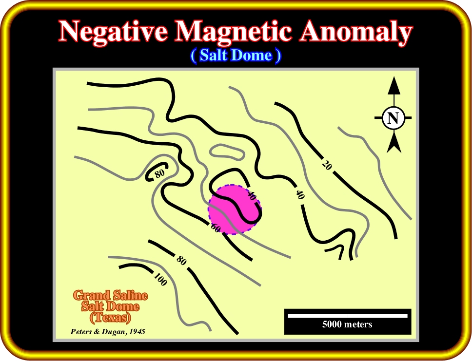
Plate 7- The negative magnetic susceptibility of salt causes a local decrease in the strength of the Earth‘s magnetic field in the vicinity of a salt dome. Readings have been corrected for large-scale variations of the magnetic field with latitude, longitude and time. The contours reflect only those variations resulting from variations in the magnetic properties of the subsurface. On this map, as expected, the salt dome (in purple) creates a negative anomaly, although the magnetic low is displaced slightly from the centre of the dome (see also Plates 15 and 16).
There are several particularities, which increase the complexity of magnetic interpretation:
a) The gravity anomaly of a causative body is entirely positive or negative, depending on whether the body is more or less dense than its surroundings.
b) The magnetic anomaly of a finite body invariably contains positive and negative elements arising from the dipolar nature of magnetism.
c) The intensity of magnetization is vectorial, while the density is scalar.
d) The direction of magnetization in a body closely controls the shape of its magnetic anomaly.
For the above reasons, magnetic anomalies are often much less closely related to the shape of the causative body than are gravity anomalies. In other words:
“Bodies of identical shape can give rise to very different magnetic anomalies”
As in other potential methods, the interpretation can be:
(i) Direct or
(ii) Inverse (Indirect)
Limiting depth is the most important parameter derived by direct interpretation. It may be deduced from magnetic anomalies by making use of their property of decaying rapidly with the distance. The inverse or indirect interpretations of magnetic anomalies are made to match the observed anomaly with that calculated for a model by iterative adjustments to the model.
The sequence of a magnetic interpretation can be summarized as follows:
a) Magnetic Anomaly (Plate 8)
About 90% of the Earth‘s field can be represented by the field of a theoretical magnetic dipole at the centre of the Earth inclined at about 11°5 to the axis the rotation.
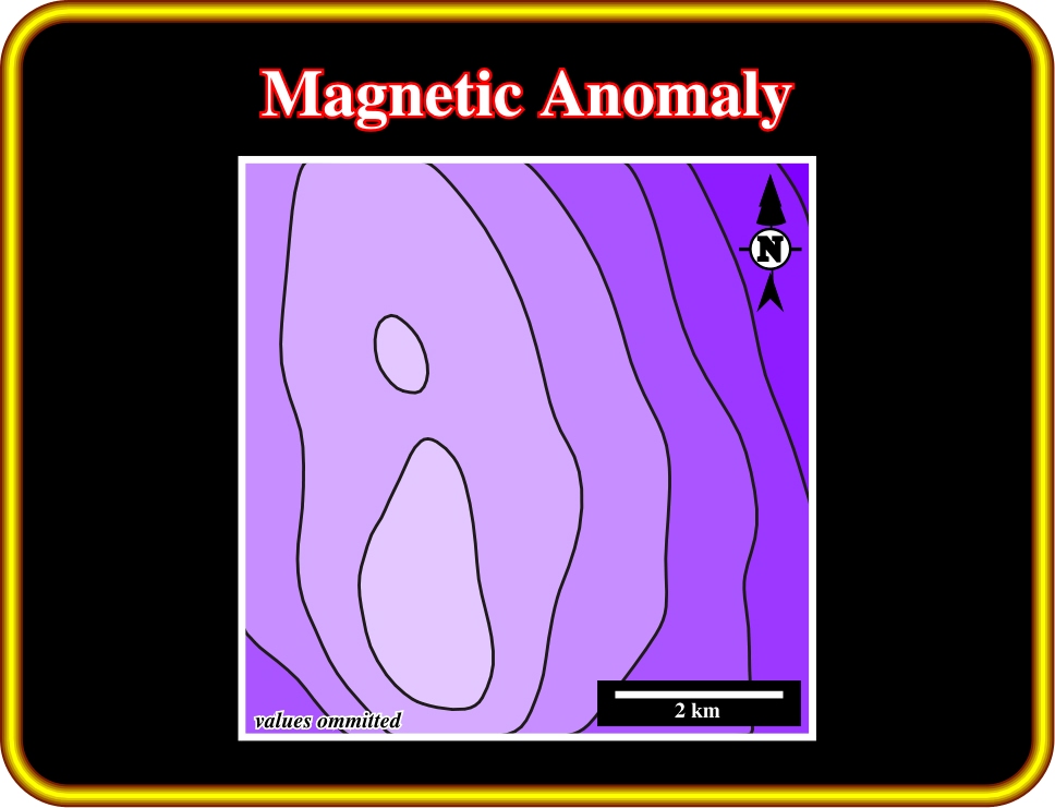
Plate 8- This map illustrates a magnetic anomaly. It represents the intensity of the Earth’s Magnetic field corrected for regional field (dipole effect) and diurnal (HF variations) effects. Magnetic anomalies are the difference between observed and corresponding computed values or the difference from the general surrounding values. Such differences are often induced by geological features.
- The magnetic moment of this fictitious geocentric dipole can be calculated from the observed.
- If this dipole is subtracted from the observed magnetic field, the residual field can be approximated by the effects of a second smaller dipole.
- The process can be continued by fitting dipoles of ever decreasing moment until the observed geomagnetic field is simulated to any required degree of accuracy.
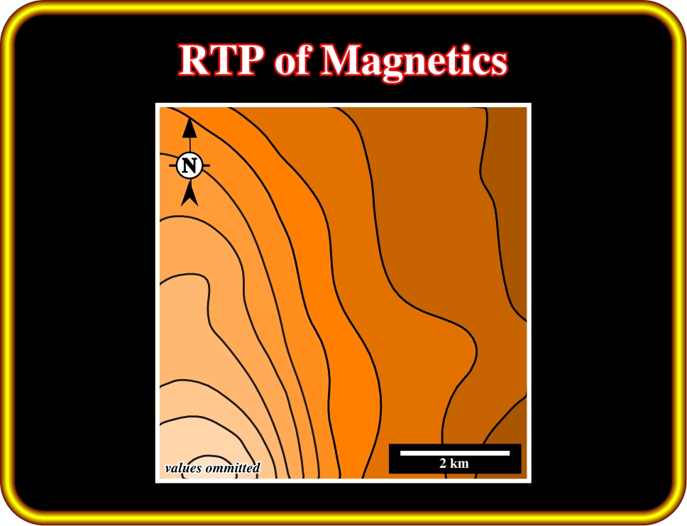
b) Reduction to the Pole (RTP) of Magnetics (Plate 9)
Reduction to the pole involves the conversion of anomalies into their equivalent form at the north magnetic pole. This process usually simplifies the magnetic anomalies, as the ambient field is then vertical and bodies with magnetizations which are solely induced. The existence of remnant magnetization, however, commonly prevents reduction to the pole from producing the desired simplification in the resultant pattern of magnetic anomalies.
Plate 9- A reduction to the pole (RTP) map of magnetics, as the one illustrated above, corresponds to the conversion of the anomalies into their equivalent form at the north magnetic pole. This process usually simplifies the magnetic anomalies (Plate 8).
c) Reduction to the Equator (RTE) of Magnetics (Plate 10)
In the northern hemisphere, the magnetic field generally dips downward the north and becomes vertical at the north magnetic pole. In the south hemisphere the dip is generally upward toward the north. The line of zero inclination approximates the geographic equator, and is know as the magnetic equator.
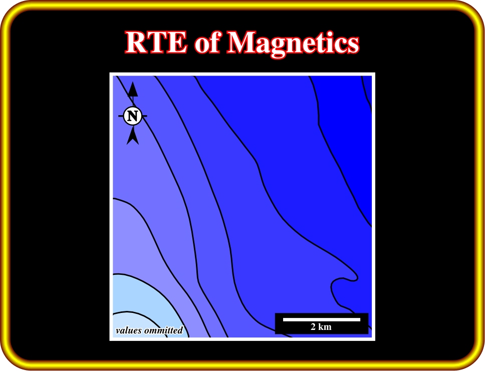
Plate 10- This RTE map of magnetics represents what the data would have looked like if the magnetic field had been horizontal (zero inclination). Comparing this map with the magnetic anomaly map (Plate 8), the advantages of a RTE map is quite evident.
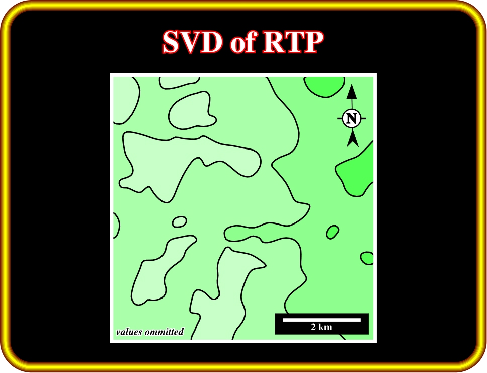
d) Second Vertical Derivative (SVD) of RTP (Plate 11)
In geophysics, derivative maps are maps of one of the derivatives of a potential field, such as the Earth’s gravity or magnetics. The more frequent derivative maps are those of the second vertical derivative (second-derivative map), which strongly enhance the morphology of the maps and so a more accurate location of the anomalies.
Plate 11- the second vertical derivative (SVD) of the reduction to the pole (RTP) map enhances subtle magnetic anomalies, which can later be corroborated or not by geological data. Enhancement of classic potential fields allows a better localization of the sources. Do not forget that the derivative of a curve is its tangent. During the night, when you drive your car in a mountainous road, the light of the headlights gives the first derivative of the road, that is to say, its inclination.
The derivative of a function, as the reduction to the pole, expresses the rate of change of that function. Indeed, on the graph of the curve y = f(x), the derivative at a given point x is equal to the slope of the tangent line at the point [x, f(x)].
Admittedly, as illustrated on Plate 11, a derivative map enhances the anomalies, which allows a finer location of the magnetic bodies.
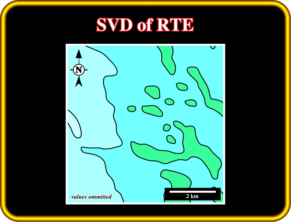
e) Second Vertical Derivative (SVD) of RTE (Plate 12)
Second vertical derivative of the reduction to the equator maps, as that illustrated on Plate 12 are often made to facilitate the recognition of subtle magnetic anomalies.
Plate 12- This map represents the second vertical derivative (SVD) of the reduction to the equator (RTE) of the magnetic anomaly (see Plate 8), which enhancing the potential field switch order a better localization of the magnetic source. To understand such enhancements suppose a long quite flat road, in which several bumpers were put in place by the local police. When driving during the daytime, the bumpers, when not painted, are difficult to locate. However, when driving during the night, they are easily located by the abrupt changes of the lights of headlights of the car moving in opposite direction (first derivative of the road).
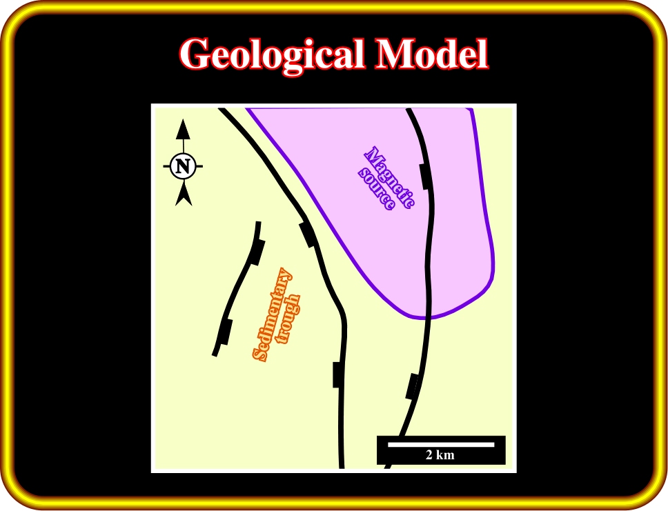
f) Magnetic Interpretation (Plate 13)
In magnetic interpretations, the problem of ambiguity is the same as for gravity. The same inverse problem is encountered. All external controls on the nature and form of the causative body must be employed to reduce the ambiguity. In other words, the same magnetic anomaly can be induced by different sources. Consequently, magnetic surveys are used in the early stage of petroleum exploration when different geological conjectures are advanced to be later tested, i.e., criticized.
Plate 13- As illustrated, a monocline geological model dipping westward with a small sedimentary trough, striking North-South and located in the western part of the map, is corroborated by the previous magnetic maps (Plates 8 to 12). Significant normal faults striking roughly north-south, seem to have lengthened the sediments. A magnetic source is likely in the north-eastern area. The proposed geological model must be tested by gravimetric and finally by seismic and subsurface data.
Summing up :
(i) Magnetic anomaly maps suggest the overall geological grain of an area, i.e, the orientation of basement highs and lows is generally apparent.
(ii) Faults may show up (close spacing or abrupt change of contours)
(iii) Sometimes, magnetic maps are used to differentiate basement (igneous and metamorphic rocks devoid of porosity) from the sedimentary cover that may be prospective. However, such a differentiation is just possible when there is a sharp contrast between the magnetic susceptibility of the basement and cover and where this contrast is laterally persistent.
(iv) Magnetic anomaly maps are also useful in petroleum exploration for indicating the presence of igneous plugs, intrusive rocks, or lava flows, i.e. areas normally avoided in the search for hydrocarbons.
(v) Seismically delineated “reef” have often been drilled and finally interpreted as igneous intrusions or volcanic plugs. A quick check of a magnetic map would indicate the presence of a magnetic anomaly and suggest an igneous intrusion rather than a reef.
In conclusion:
Magnetic surveys are a quick and cost effective way of defining broad basin architecture. Though, they can seldomly be used to located drillable petroleum prospects.
to continue press
![]()