According to Nettleton (1976), any conceivable property or process, which can be measured or carried out at above the surface and which is affected by the nature of rocks through a cover of hundreds to many thousands of feet of intervening rocks, may be made the basis of a method of geophysical prospecting.
Fundamentally, there are two main families of geophysical surveying (Kearey and Brooks, 1993):
(i) Natural Field Methods
They utilize the gravitational, magnetic, electrical and electromagnetic fields of the Earth and look for local perturbation in these naturally occurring fields that may be caused by concealed geological features.
(ii) Artificial Field Methods
They involved the generation of local electrical or electromagnetic fields that may be used analogously to natural fields. In the most important group of geophysical methods, the generation of seismic waves and their propagation velocities and transmission paths through the subsurface are mapped to provide information on the distribution of the geological boundaries at depth.
A wide range of physical surveying methods exists. For each method there is an operative physical property to which the results are sensitive :
a) Seismic Method
It measures the travel times of reflected or refracted seismic waves using as operative properties the density and elastic moduli, which determine the propagation velocity of seismic waves.
b) Gravity Method
It measures the spatial variations in the strength of the gravitation field of the Earth. The operative physical property is the density.
c) Magnetic Method
It measures the spatial variations in the strength of the magnetic field. The operative physical property is the magnetic susceptibility and remanence.
d) Radar Method
It measures the travel times of reflected radar pulses. The operative physical property is the dielectric constant (the dielectric constant k is the relative permittivity of a dielectric material, which is an electrical insulator that can be polarized by an applied electric field or a substance in which an electric field can be maintained with a minimum loss of power).
In the majority of geophysical survey methods, geoscientists are mainly interested in geophysical anomalies, i.e., local variations in the measured parameter relative to some normal background value. Such variations are attributable to a localized subsurface zone of distinctive physical properties and possible geological importance. However, geophysical interpretation is quite ambiguous.
There are two kind of problems in geophysical surveying:
- If the internal structure and physical properties of the Earth were precisely known, the magnitude of any particular geophysical measurement taken at the Earth‘s surface could be predicted uniquely. Thus, for example, it would be possible to predict the travel time of a seismic wave reflected off any buried layer or to determine the value of the gravity or magnetic field at any surface location (P. Kearey and M. Brooks, 1993).
- However, often, in geophysical surveying, the problem is the converse of the above, namely, to deduce some aspects of the Earth’s internal structure on the basis of geophysical measurements taken at (or near to) the Earth’s surface.
The former type of problem is known as a direct problem, the latter as an inverse problem. Whereas direct problems are theoretically capable of unambiguous solutions, inverse problems suffer from an inherent ambiguity or non-uniqueness of conclusions that can be drawn.
Let’s see the examples proposed by P. Kearey and M. Brooks (1993):
a) Direct Problem
The travel time of an echo-sounding is measured and converted into a water depth multiplying the travel time by the velocity with which sound waves travel through water (± 1500 m/s). Thus an echo time of 0.10 s indicates a path length of 0.10 x 1500 = 150 m or a water depth of 150/2 = 75 m, since the pulse travels down to the sea bed and back up to the transducer located in the ship.
b) Inverse Problem
Using the same principle, a simple seismic survey may be used to determine the depth of a buried geological interface (e.g. the top of a limestone layer or basement). This would involve generating a seismic pulse at the Earth’s surface and measuring the travel time of a pulse reflected back to the surface from the top of the limestone or top of basement. However, the conversion of this travel time into a depth requires knowledge of the velocity with which the pulse travel along the reflection path. Unlike the velocity of sound in water, this information is generally not known. If a velocity is assumed, a depth estimate can be derived, but it represents only one of many possible solutions.
Although the degree of uncertainty in geophysical interpretation can often be reduced to an acceptable level by taking additional field measurements, the problem of inherent ambiguity cannot be overcome. The general problem is that significant differences from an actual subsurface geological situation may give rise to insignificant or immeasurable small differences in the quantities actually measured during a geophysical survey. Since a unique solution cannot, in general, be recovered from a set of field measurements, geophysical interpretation is concerned either to determine properties of the subsurface that all possible solutions share or to introduce assumptions to restrict the number of admissible solutions (Parker, R. L., 1977).
Practically, all geophysical search for hydrocarbon exploration depend on a very few basic physical principles :
(i) Elastic waves ;
(ii) Magnetics ;
(iii) Gravity ;
which characterize the three main prospecting methods :
- Seismic methods ;
- Magnetic methods ;
- Gravimetric methods.
Seismic methods are concerned with the measurement and analysis of waveforms that express the variation of some measurable quantity as a function of distance and time. The quantity of information and, in some cases, the complexity of data processing to which these waveforms are subjected is such that the processing can only be accomplished effectively and economically by digital computers (perform calculations and logical operations with quantities represented as digits, usually in the binary number system).
The two basic parameters of a digitizing system are:
1) Sample Precision or Dynamic Rang ;
The dynamic range, which is expressed in decibel (dB), is the expression of the ratio of the largest measurable amplitude to the smallest measurable amplitude in a sample function.
2) Sampling Frequency ;
The sampling frequency is the number of sampling points in unit time or unit distance. Ex: if a waveform is sampled every two milliseconds (sampling interval), the sampling frequency will be 500 samples per second or 500 Hz.
If frequencies above the Nyquist frequency are present in the sampled function, a serious form of distortion known as aliasing occurs (the Nyquist frequency is the frequency of half the sampling frequency and Nyquist interval is the frequency range from zero to the Nyquist frequency). To overcome this problem, either the sampling frequency must be at least twice as high as the highest frequency component present in the sampled function or the function must be passed through an anti-alias filter prior to digitalization.
Gravimetric and Magnetic methods are potential field methods. They have their fundamentals in the mathematical theory of potential fields. So, gravitational or magnetic forces are, in a given direction, the derivative or rate of change, in that direction, of the gravitational or the magnetic potential.
(In these notes, we will concentrate mainly in the seismic method and particularly seismic reflection and geological interpretation. Magnetic and gravitational, i.e., the potential methods will be just briefly outlined.)
Gravimetry and Magnetics, that is to say, the potential methods are based on the potential theory. The term "potential theory" assumes that the fundamental forces of nature could be modeled using potentials which satisfy Laplace's equation (simple example of elliptic partial differential equations which solutions are called harmonic functions). The potential methods have certain elements in common. Nevertheless their applications in oil exploration are quite different :
(i) Measured gravity effects are caused by sources that may vary in depth from the grass roots down ;
(ii) Sedimentary rocks, which are the ones in which generally hydrocarbon may occur, nearly always are less magnetic than the underlying basement (usually igneous or metamorphic rocks) ;
(iii) Magnetic effects are not too influenced by the sediments. Its effects are almost the same as if the sediments were not present.
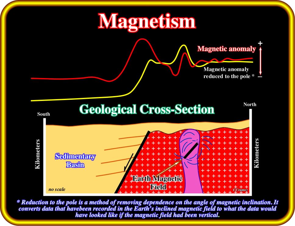
Plate 25 - This figure depicts the main principles of the magnetic method. A survey is made with a magnetometer on the ground or in the air. The survey yields local variations or anomalies in magnetic field intensity. Then, the anomalies will be compared and interpreted in relation to a geological model, as to the depth, size, shape, and magnetization of geologic features causing them. Magnetic methods are widely used in petroleum exploration, engineering, borehole, and global geophysics.
Petroleum geologists and geophysicists, often called Geoscientists or Explorationists, should not forget that these methods are deterministic, in which all facts and events exemplify natural laws (methods non-deterministic methods are non-predictive, that is to say, they are inable to objectively predict an outcome or result of a process due to lack of knowledge of a cause and effect relationship or the initial conditions), which implies an important epistemological limitation :
"Gravimetric or magnetic maps can just falsify or corroborate geological models (indirect interpretation). They cannot or should not be used to make geological interpretations "
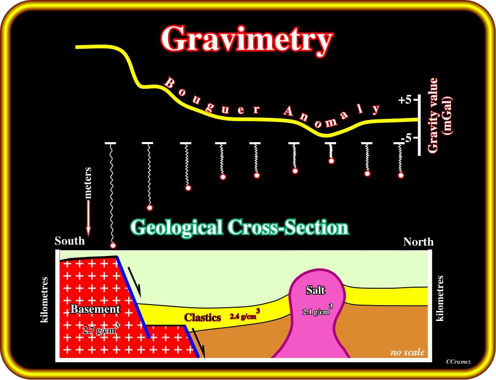
Plate 26- Gravity is usually measured in units of acceleration. In the SI of units, the standard unit of acceleration is 1 m/s2). Other units include the gal (sometimes known as a galileo, in either case with symbol Gal), which equals 1 centimeter per second squared, and the g (gn), equal to 9.80665 m/s2. The value of the gn (g) approximately equals the acceleration due to gravity at the Earth's surface (although the actual acceleration g varies fractionally from place to place). In this geological cross-section, the relatively low density of salt with respect to its surroundings renders the salt dome a zone of anomalously low mass. The Earth's gravitational field is perturbed by subsurface mass distributions and the salt dome therefore gives rise to a negative gravity anomaly with respect to surrounding areas, as illustrated in the upper part of the plate by the Bouguer anomaly. As gravimetry is a deterministic method, a priori geological interpretation is required, which, then, can be refuted or corroborated by the gravimetric data.
Gravity and magnetic processing sequences can be summarized as follows:
a) Pre-Processing :
(i) Reading / Converting Field Tapes ;
(ii) Line Definition ;
(iii) Data Editing ;
(iv) Digitizing (if unrecordable or not recorded digitally) ;
(v) Positions, Shot-points, and Time (if acquired on a seismic operation).
b) Basic Processing :
- Meter Calibration, Base Constants and Drift ;
Correction for instrumental drift is based on repeated readings at a base station at recorded times throughout the day.
- Base Station Magnetic Observation and Diurnal ;
The effects of diurnal variation may be removed in several ways. For magnetics (land), a method similar to gravimeter drift monitoring may be employed, in which the magnetometer is read at a fixed base station periodically throughout the day.
Magnetometers do not drift and base readings are taken solely to correct for temporal variation in the measured field. Magnetic effects of external origin cause the geomagnetic field to vary on a daily basis to produce diurnal variations. Under normal conditions (quiet days), the diurnal variation is smooth and regular and has small amplitude, being at maximum in Polar Regions. Disturbing days are distinguished by far less regular diurnal variations and involve large, short-term disturbances in the geomagnetic field, with big amplitudes (magnetic storms).
- Intersection Determination ;
- Misty Adjustments :
(i) Systematic Corrections ;
(ii) Random Error Correction.
- Profiling ;
- Gridding and Contouring ;
- General Reduction.
Before the results of gravity or magnetic surveys can be interpreted, it is necessary to correct them for all variations in the Earth‘s potential fields :
- International Gravity Formula ;
It is a formula expressing theoretical gravity on the surface of a specified reference ellipsoid as a function of latitude.
- Earth’s Normal Magnetic Field ;
The International Geomagnetic Reference Field (IGRF) defines the theoretical dipolar undisturbed magnetic field related to neck at any point on the Earth's surface. In magnetic surveying, the IGRF is used to remove from magnetic data those magnetic variations attributable to this theoretical field.
- Correction Sun / Moon motion ;
- Eötvös Correction ;
In gravity measurement, on a moving platform (ship or aircraft) a correction, for centripetal acceleration caused by east-west velocity over the surface of the rotating Earth, is necessary, since the Eötvös effect is the change in perceived gravitational force caused by the change in centrifugal acceleration resulting from eastbound or westbound velocity (http://en.wikipedia.org/wiki/Eötvös_effect).
- Free Air Correction;
This correction corresponds to the natural decreasing of the field with elevation, i.e., the distance between observation point and the geoid (an imaginary surface that coincides with mean sea level in the ocean and its extension through the continents - http://dictionary.reference.com/browse/Geoid.)
- Bouguer and Terrain Corrections ;
The Bouguer correction is a correction made to gravity data for the attraction of the rock between the station and the datum elevation (commonly sea level). If the station is below the datum elevation, for the rock missing between the station and the datum, the Bouguer correction is 0.01276 ph mgal/ft or 0.04185 ph mgal/m, where p is the specific density of the intervening rock and h the difference in elevation between the station and datum.
Terrain corrections should be applied if the actual topographic or bathymetric surface deviates significantly from the infinite Bouguer slab. For land and underwater stations, this correction is positive because both high areas above the station and low areas below it causes a lower gravity reading than would have been observed if the land were flat. For the sea stations over relatively deep water, a negative correction may be required because of the positive influence surrounding rocks above the station water depth.
Terrain correction can be made either manually or by computer by dividing the topography into compartments and summing the individual effects at each station. This requirement can add significantly to the cost of processing gravity data.
On geological tentative interpretations of a seismic data (Plate 27), interpreters must avoid the temptation to envisage seismic sections as straightforward images of geological cross-sections.
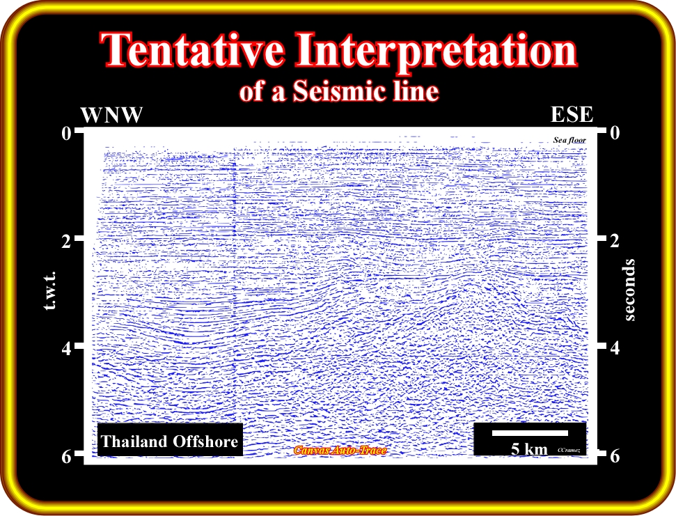
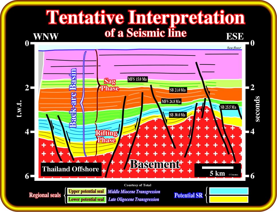
Plate 27- Geological tentative interpretations of seismic lines require the knowledge of the global and regional geological context of the areas where they were shot. This tentative interpretation of a line shot in the Thailand offshore, must fit with the general characteristics of back-arc basins, in which a tectonic sag phase overlies a rifting phase. Geoscientists should not forget that the vertical scale is in time (two-way times) and the horizontal scale metric. On the other hand, with few exceptions, all seismic markers correspond to chronostratigraphic lines, that is to say, interfaces between relatively thin (20-60 m) sedimentary intervals. Some of these interfaces correspond to unconformities (erosional surfaces created by a significant relative sea level fall, as SB 21.0 Ma or SB. 30 Ma in this tentative) and others to downlap surfaces (see later), which separate sedimentary transgressive episodes (backstepping geometry) from regressive episodes (forestepping or progradational geometry).
Geoscientists should not forget that:
1) The vertical scale is in time and not depth.
In addition, on the tentative interpretation depicted above (Plate 27), it is important to notice that :
a) Seismic surfaces are defined by reflection terminations ;
b) The basement, in this particular instance, is an old folded belt ;
c) The geological global context is that of an episutural basin ;
d) Above the substratum, there is a back-arc basin ;
e) The back-arc basin is composed of a rifting (rift-type basin) and a sag phase ;
f) Reflectors discontinuities have been interpreted as fault planes ;
g) The more likely potential source-rocks were deposited in the rift-type basin ;
h) The potential sealing-rocks are associated with the transgressive interval of the sag phase ;
i) The chronostratigraphic calibration is based on the Vail's Neogene stratigraphic signature.
2) The seismic resolution is generally higher than 50-60 m.
A key requirement for successful application of seismic stratigraphic principles is a good understanding of the resolution of the seismic method. Generally, geological intervals thinner than 30-60 m are under the vertical seismic resolution (Plate 28).
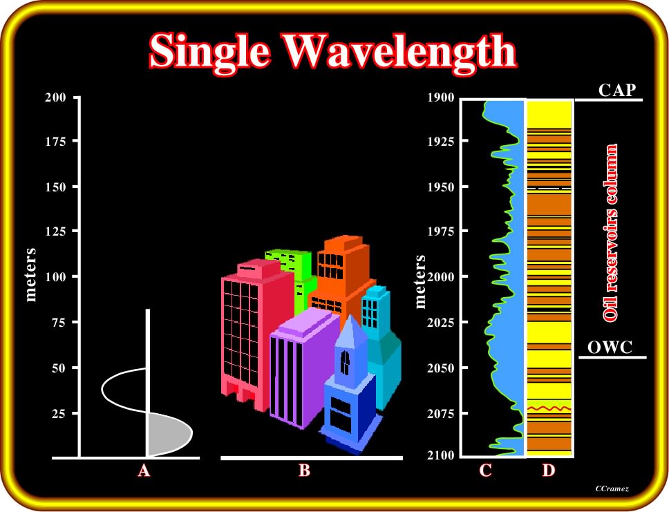
Plate 28- This plate illustrates the vertical comparison between (A) a single cycle sine wave of 30Hz in a medium of velocity 6000 fps (or 60 Hz; 12000 fps) ; (B) Buildings and (C) Electrical log through an oil field. Geoscientists must be quite careful when proposing the interpretation of small geological bodies, as channels, point bars, etc., which in the majority of the cases are under seismic resolution. Seismic resolution is the ability to distinguish separate features, that is to say, the minimum distance between 2 features so that the two can be defined separately rather than as one. Normally, geoscientists take the resolution in the vertical sense, but there is also a limit to the horizontal width of an object that we can interpret from seismic data. The seismic "measure" is a wavelength. In order for two nearby reflective interfaces to be distinguished well, they have to be about 1/4 wavelength in thickness (Rayleigh Criterion). This is also the thickness where interpretation criteria change. For smaller thicknesses than 1/4 wavelength we rely on the amplitude to judge the bed thickness. For thicknesses larger than 1/4 wavelength we can use the wave shape to judge the bed thickness. Near the earth's surface (upper 10 meters depth), roughly, the values of velocity, frequency and wavelength (Velocity = Frequency x Wavelength.) are 1000 m/s, 100 Hz, wavelength = 10 m, while in deep earth, (5000 meter depths) they are 5000 m/s, 20 Hz, wavelength= 250 m. In other words, geoscientists can recognize a given geological body near surface but not in the deep parts. This is particularly true in deltaic environments. In fact, as the thickness of a delta (not a stacking of deltas) is hardly more than 60 meters, the recognition of deltaic progradations is probable in the uppermost levels of a seismic line but not in the deep parts. Actually, in the majority of the cases, when a geoscientist recognizes a progradational interval, at 2-3 seconds depth, the progradaitions correspond rather to continental slopes than deltaic slopes.
All interpreters need to take into account both vertical and lateral resolution :
- Vertical resolution ;
It can be defined as the minimum vertical distance between two interfaces needed to give rise to a single reflection that can be observed on a seismic section. This is governed by the wavelength of the seismic signal.
- Lateral resolution ;
It is determined by the radius of the Fresnel zone, which itself depends on the wavelength of the acoustic pulse and depth of the reflector. Seismic energy travels through the subsurface and comes into contact with the reflecting surfaces over discrete areas much in the same way that a spotlight travel through the darkness and illuminates a particular area. The energy travels as wave fronts, and the region on the reflector, where the seismic energy is reflected constructively, is known as Fresnel zone.
In non-migrated seismic data, lateral resolution is dependent on :
(i) Seismic bandwidth ;
(ii) Interval velocity ;
(iii) Travel time to the reflector.
The procedure of migrating seismic data considerably enhances resolution. However, for two-dimensional migration there is still the problem of the line orientation relative to actual dip. This is resolved on 3D data.
For migrated data, lateral resolution depends on :
(i) Trace spacing ;
(ii) Length of the migration operator ;
(iii) Time/depth of the reflector ;
(iv) Bandwidth* of the data.
* The bandwidth is the measure of the width of a range of frequencies, measured in hertz
In fact, the frequency of reflected signals decreases with increasing time/depth (t.w.t.). The main causes of this effect aren :
A) Absorption
Absorption is essentially a loss of energy by conversion into heat. We can picture this happening on the microscopic scale :
Particle motion during passage of the seismic wave causes grains to slide against one another, and friction between the grains causes energy loss.
In a given rock, there is generally a constant fractional energy loss per cycle of the seismic wave. There is a constant fractional loss per wavelength.
Higher frequencies are attenuated more than lower ones over a given path. High frequencies will be quite strongly absorbed in traversing a path typical of reflection prospecting, leaving a signal whose dominant frequencies are a few tens of Hz. Earth is a low-pass filter.
B) Effect of short-period multiples
On the earth there is a good deal of layering between the source and the deep reflector. A signal can therefore bounce backward and forward between any two reflectors including land surface, seabed and sea surface a number of times, and perhaps arrive back at the receiver at nearly the same time as the deep reflector signal. These secondary signals or multiples must be eliminated from our record. Short-period multiples also cause a decrease of frequency with travel-time.
Briefly, part of the seismic energy is delayed on its path by reverberation (persistence of energy in a particular space after the original source is no longer) between closely spaced reflecting interfaces. Thus an initially sharp pulse (even if we could produce one) will be smeared out in its passage trough the earth, in effect leading to a slow decrease of frequency with depth.
3) Reflections are not always chronostratigraphic lines
The great majority of the seismic markers correspond to chronostratigraphic lines. Such analogy was recognized by the Exxon's geophysicists, which conceived seismic stratigraphy. Peter Vail summarized the origin of the birth of seismic stratigraphy as follows:
“When Exxon in the 60‘s explored the offshore Portuguese Guinea (now Guinea Bissau) three wells had been drilled. The most landward well had hit the top of major Cretaceous reservoir sand, overlying an unconformity with Paleozoic rocks below. When the second well was drilled down-dip, it was predicted that this sand would be high in the well, but it was actually encountered much lower. As a result, it was a dry well. A similar experience occurred in the third well. Then Exxon explorationists looked at the seismic section, and saw that the reflection from the top of the sand in the first well was two reflection above the reflection of the top of the sand in the second well and even higher in the third well. There was no miscorrelation of the seismic data with the well-logs and the micropaleontologists confirm that the seismic reflections were following the time lines. The pattern correlation of the well-log marker horizons showed that the real physical surfaces cross the facies of time-transgressive rock units, suggesting that the seismic reflections do not follow massive time transgressive formational boundaries where strong impedance occur, but instead they follow the detailed bedding pattern or the real physical surfaces in the rocks. Thus, they cross time-transgressive facies and rock-formation boundaries, which are not continuous physical surfaces. At the time, this was revolutionary basic driving concept. It provided a new driving concept for interpreting seismic data”.
However, on a seismic line, it is common to recognize seismic markers that do not correlate with chronostratigraphic lines (Plate 29).
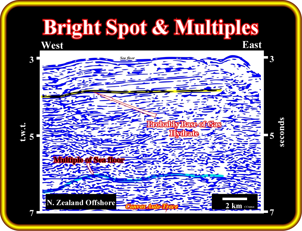
Plate 29- This tentative interpretation of seismic line from New Zealand offshore shows a bright spot (in yellow), which can be interpreted as the lower surface of a gas hydrate accumulation (mineral compound CH4 and water). Basal hydrate reflectors commonly occur in sub-bottom depth, with increasing water depth, because of decreasing temperature of water above the sea floor. The term bright spot is used to named a seismic amplitude anomaly or high amplitude that can indicate the presence of hydrocarbons. They result from large changes in acoustic impedance and tuning effect (tuning is the process a system to to improve performance). For instance, the tuning of a receiver or an oscillato (adjusting to a desired frequency)., such as when a gas sand underlies a shale, but can also be caused by phenomena other than the presence of hydrocarbons, such as a change in lithology. Amultiple reflection of the sea floor is probably at around 6 seconds (t.w.t.).
Among the non-chronostratigraphic reflectors, we can differentiate
- Multiple reflections, reverberation or simply multiples ;
- Ghost reflections ;
- Water layer reverberations ;
- Short-path multiples ;
- Long-path multiples ;
- Bright spots (Plate 29), Bottom Reflectors (Plate 30), etc.
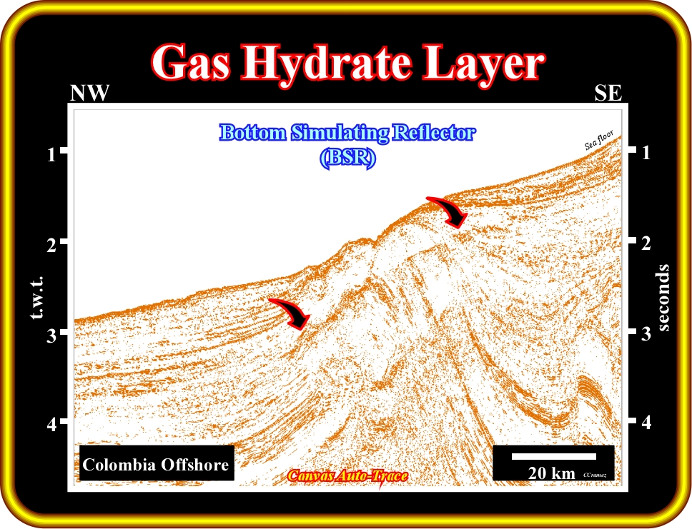
Plate 30- On this tentative interpretation (the reflectors are underlined by small strokes) of seismic line from offshore Colombia, a bottom simulator reflector is easily recognized. The gas hydrate stability zone (GHSZ) occurs in oceanic sediments over the first few hundred meters below sea floor. In this zone, any methane from organic material, including any seepage from below, is converted into solid hydrate, and is locked in place in the sediments. The origin of the methane is poorly understood, with even its biogenic origin being challenged. There are three main areas of gas hydrate occurrences : (i) The regions of continuous onshore permafrost ; (ii) The regions of subsea permafrost within the arctic shelves and (iii) The oceanic regions of the outer continental margin. The first and the third regions are currently characterized by fairly stable conditions. Due to gas hydrate stability zone dynamics, changes in the concentration of greenhouse gases can be initiated more likely in the region of continental shelves with gas hydrates (http://www.cgc.uaf.edu/Newsletter/gg4_2/gas.html).
Particular care must be taken to distinguish gas hydrates bottom reflectors from ordinary seabed multiples (Plate 29). On this subject it is interesting to summarize the composition, occurrence and economic significance of gas hydrates (Selley, R., 1998):
- Gas hydrates are compounds of frozen water that contain gas molecule ;
- The ice molecules themselves are referred to as clathrates ;
- Physically, hydrates look similar to white, powdery snow and exhibit two types of unit structure;
- They occur only in very specific pressure temperature conditions ;
- The pressure required for stability increasing logarithmically for linear thermal gradient ;
- They are stables at high pressures and low temperatures ;
- The pressure required for stability increasing logarithmically for linear thermal gradient ;
- Gas hydrates have been found in sediments of many oceans around the world ;
- They have been recognized from bright spots on seismic lines in water depths of 1000 to 2500 m (N. Sea) and in water depths of 1000 to 4000 m (North Atlantic);
Gas hydrates have been attributed to a shallow biogenic source. However, a crustal inorganic origin has been postulated, based on analysis of their carbon and helium isotope ratios:
- It is probable that methane comes from three sources :
(i) Some may be derived from the mantle ;
(ii) Some may be derived from the thermal maturation of kerogen ;
(iii) Some may be derived from bacterial degradation of organic matter at shallow burial depths.- The presence of gas hydrates can be suspected, but not proved from seismic data ;
- The lower limit of hydrate-cemented sediment is often concordant with bathymetry (Plate 29 & 30) ;
- The velocity contrast between the gas-hydrate cemented sediment and underlying non cemented sediment is large enough to generate a detectable reflection horizon ;
- The bottom-simulating reflector (BSR) may appear as a bright spot, which cross cuts bedding-related reflectors ;
- The presence of gas hydrates can only be proved, however, by engineering data. They have high resistivity and acoustic velocity, coupled with low density.
- Detailed studies have been carried out on 12 selected areas of known gas occurrence. These studies have revealed that these areas contain well in excess of 100.000 Tcf of gas within the hydrate cemented sediment, and more than 4.000 Tcf of gas trapped beneath the hydrate seal (Selley, 1998) ;
Estimated Gas Resources in Gas Hydrates
(Krason, J, 1994)
Area studied.....................................................................1 m hydrate zone
Tcf................................m3
Offshore Labrador--------------------------------------------------25-------------------------0,71 T
Baltimore Canyon---------------------------------------------------38-------------------------1,08 T
Blake Outer Ridge--------------------------------------------------66-------------------------1,88 T
Gulf of Mexico-------------------------------------------------------90-------------------------2,57 T
Colombia Basin----------------------------------------------------120-------------------------3,42 T
Panama Basin--------------------------------------------------------30-------------------------0,85 T
Middle America Trench-------------------------------------------92-------------------------2,62 T
Northern California--------------------------------------------------5-------------------------0,14 T
Aleutian Trench-----------------------------------------------------10-------------------------0,28 T
Beaufort Sea--------------------------------------------------------240-------------------------6,85 T
Nankai Trough-------------------------------------------------------15------------------------0,42 T
Black Sea---------------------------------------------------------------3-------------------------0,08 T
- Unfortunately, gas hydrates present considerable production problems that have yet to be overcome. These problems are due, in part, to the low permeability of the reservoir and, to chemical problems concerning the release of gas from deep crustal zones ;
- Clathrates deposits may be of indirect economic significance, however, by acting as cap rocks ;
- Because of their low permeability, they form seals that prevent the upward movement of free gas ;
- Some gas is produced from gas hydrates in western Siberia, where they pose some interesting engineering problems.
- Gas hydrates may have considerable importance in understanding climatic changes ;
- Relative sea level falls can induce sudden release of gas may trigger mud volcanoes and pock-marks on the sea bed, pingos in permafrost, as well as large turbiditic currents ;
- The huge increase of greenhouse gas into the atmosphere may be responsible for the sudden increase in global temperature and carbonate deposition (Gaia Theory).
to continue press