Page11

Universidade Fernando Pessoa

Porto, Portugal

Volume Problem
in
Real Crustal Deformation

B- Imbricated Curvilinear-Planar Faults

In imbricated normal curvilinear-planar faults the extension is so important that some hangingwalls can be completely detached from the updip footwall (Fig. 139).

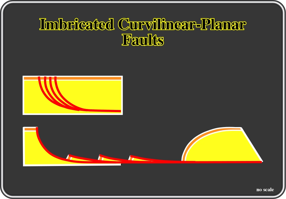
Fig.139- When extension is big enough imbricated normal curvilinear faults become almost planar. The displacement along each fault is approximately equal to the length of the fault-blocks, as corroborated by the seismic interpretation illustrated in fig. 140.

Fig. 140- Imbricated curvilinear-planar normal faults can be recognized on the seismic line from offshore Angola. Salt tectonics induced large extension with formation of pre-raft and rafts structures, as well as depocenters in the overburden (post salt sediments).

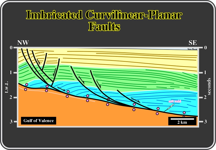
Fig. 141- Imbricated normal curvilinear faults created extension over a mobile substratum (Messinian evaporites) are quite frequent in the Gulf of Valence as depicted in this seismic interpretation.

C- Depth of Décollement Surfaces

The depth of the détachment surfaces in which the curvilinear faults flatten and die can be calculated quite easily as illustrated in fig. 142.

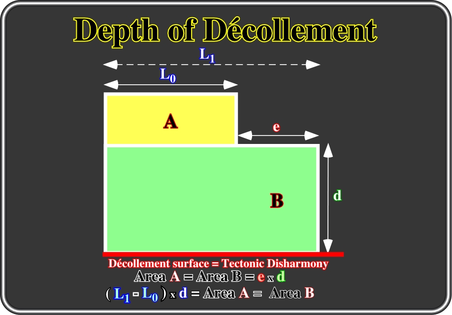
Fig. 142 - An undeformed sedimentary interval L0 is lengthened to L1. Its thickness decreases to a value d. However, the volume of sediments is kept constant. As the volumetric Goguel’s law can be considered as a bidimensional, one can say that area A is equal to area B. The extension e is given by the difference between L1 and L0. The depth of the décollement surface (d) can be determined by dividing the area A or B by the amount of extension (e).

Fig. 143- In this interpretation, the décollement surface, where the normal curvilinear faults, exhibiting a westward vergence, flatten, is not visible on the seismic line. However, its depth can be calculated by the excess area method, dividing the excess area, which is equal to the extended area, by the amount the extension e (L1-L0), as illustrated below.

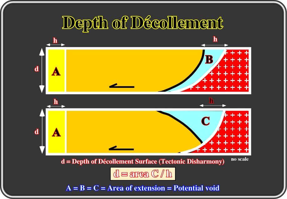
Fig. 144- The depth of the tectonic disharmony, in which curvilinear normal faults die, can be calculated by dividing the area of extension by the heave of the fault (h).

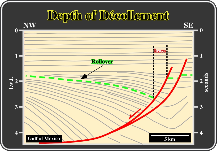
Fig. 145- In a normal curvilinear fault, the geometry of the fault plane can be calculated by knowing the geometry of downthrown block (rollover) and the heave of the fault, as illustrated in figure 144.

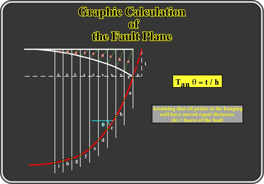
Fig.146- In a normal curvilinear fault, knowing the geometry and the rollover (hangingwall) and the heave of the fault, and assuming that all points of the hangingwall have move of equal distance, one can calculate the geometry of the fault planes in depth, as depicted.

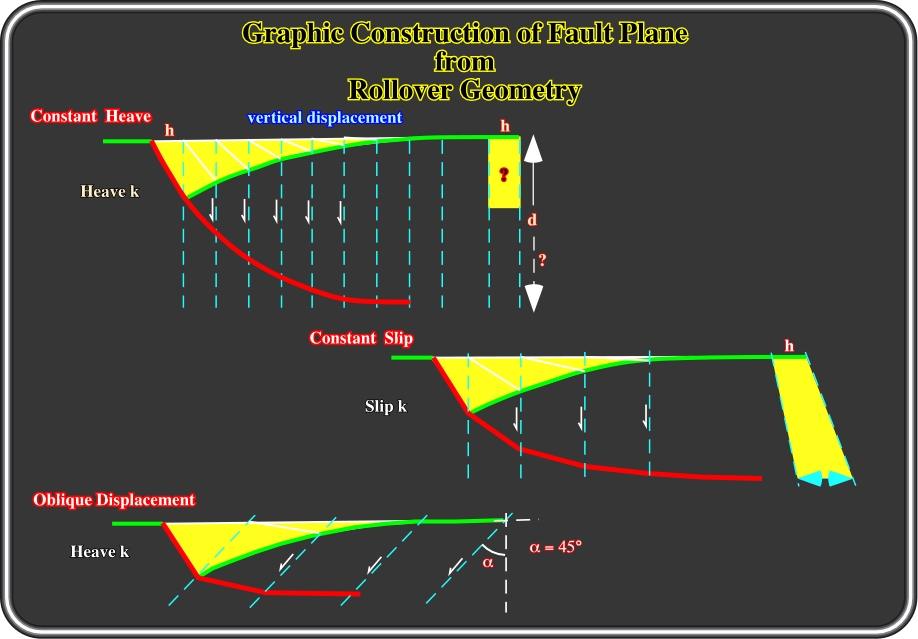
Fig. 147- Three different graphic methods can be used to construct the trace of the listric fault plane using the geometry of the rollover: (i) Constant heave, (ii) Constant Slip and (iii) Oblique displacement.

Fig. 148- Assuming two faulted blocks and two detachment planes with associated listric ramps, the volume problems created by the horizontal displacement of the hanging-wall, relatively to the footwall, are solved by the development of two hanging wall synclines at the vertical of the ramps.

Fig. 149- The deformations of the hangingwall solving volume problems are summarized in these sketches. It is interesting to notice the development of rollover-drag in the hangingwall whenever there is a sharp lithologic change in the footwall. Indeed, when a fault is pre-compaction, a lithological change in the footwall will be emphasized by a change in the dip of the fault plane.

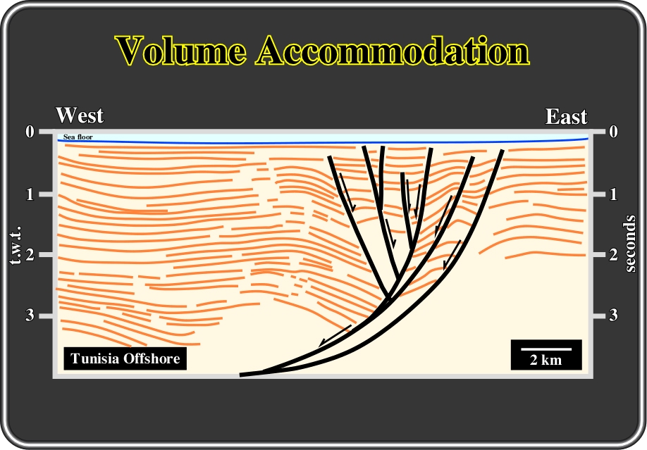
Fig. 150- This interpretation of a seismic line from offshore Tunisia, illustrates the hanging wall deformations developed to fill the space created by extension. In this particular example, several accommodation faults (antithetics and synthetics) were necessary to extend the sediments in order to fill the space created by extension (void problem).

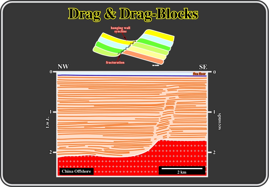
Fig. 151- Often, the hanging wall syncline is not deformed as illustrated in the sketch above. Indeed, in certain seismic lines, as in the interpretation above, one can say that the hanging wall syncline is reduced to a simple fractured zone dipping downward.

Fig. 152- Notice that generally there is not a seismic marker associated with fault planes. Seismically, fault planes correspond to seismic surfaces characterized by a sharp discontinuity of the seismic markers. Gouge zones as illustrated above are visible on the seismic lines only when their thickness is above the seismic resolution.

Fig. 153- Hanging wall synclines can be utterly complex particular in association with “X” faults, that is to say, when fault planes are cut and displaced by younger faults. In these complex faulted areas, very often, graben structures overly horst structures. Indeed such a superposition, in the same vertical area, is the best way to identify X faults on cross-section and seismic lines.

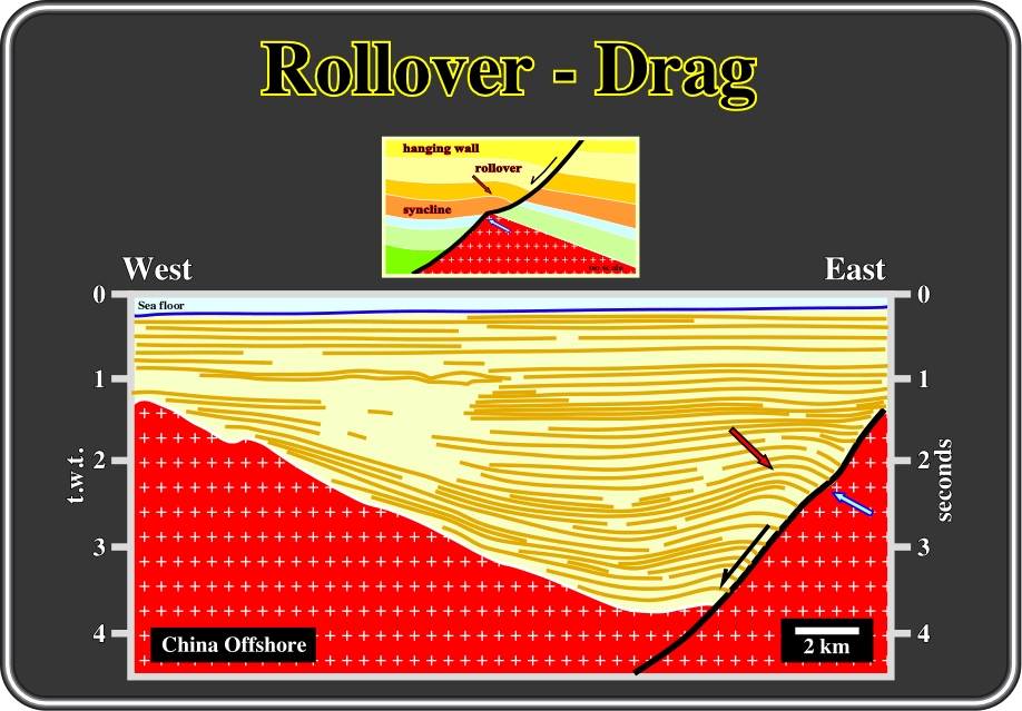
Fig. 154- On this interpretation of a seismic line from the Pearl River Mouth basin, in the footwall, the limit between the Tertiary sediments and the infrastructure (Paleozoic or Precambrian) induced a rollover in the hanging wall, which is often taken as a target by petroleum geologists. One should not forget that a rollover is not an anticline. A rollover is an antiform, that is to say, an extensional structure affected by small normal faults, in other words one can say that there is not structural traps (four way dips) associated with rollovers.

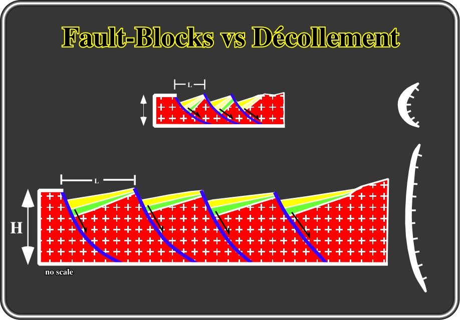
Fig. 155- Volume problems control the geometry of fault planes and fault-blocks. There is a typical relationship between the length of the fault blocks (L), the rotation of the sediments in the hanging blocks, and the depth of the detachment plane and the surface geometry. In other words, the larger the fault-blocks, the deeper the detachment planes are and the higher the rotations of the hanging wall blocks are . On the other hand, one can say that the higher the rotation of the hanging wall the more curvilinear the surface geometry of the faulted plane will be.

c.5.b- Faults without or with Rotation of the Fault-blocks

Here, we will review mainly the process of folding at bends of extensional faults, that is to say, extensional fault-bend folding. Indeed, as illustrated below, when faults form, they often develop bends, or changes in orientation.

Fig. 156- These sketches show an example of a normal fault with a flattening bend prior to the development of significant displacement along the fault. If rocks were sufficiently strong, then continued fault movement would open a void. However as said previously, in the earth, rocks must deform to fill the void as the hangingwall block moves past the fault bend. Rocks fold to accommodate this space problem: (i) the inactive axial plane moves with the hangingwall block, (ii) the active axial plane is pinned to the fault bend and remains stationary relative to the footwall block, (iii) the rocks fold continuously as they move through the active axial plane, (iv) the rocks can fold by one or more of any possible deformation mechanism, including grain sliding and minor faulting.

Fig. 157- In the model proposed by Xiao and Suppe (1991), extension is accomplished by Coulomb shear (bulk frictional slip, like in a pile of sand) not by flexural-slip of bedding (like bending a deck of cards). Therefore, this model is applied in exactly the same manner when analysing basement rocks, massive sedimentary units, thinly layered sedimentary rocks or unconsolidated sediments because bedding is passive during Coulomb shear. The dip-angle of the fold axial planes is equal to the Coulomb shear-angle of the deformed rocks or unconsolidated sediments. The dip-angle is therefore fixed and is unrelated to the orientation of the fault segments on either side of the bend. Note that axial planes can be reoriented by later deformation. Material conservation requires that the cross-sectional area of the extended fold panel remains constant, in 2-dimensional models. In three dimensions volume is conserved. The Coulomb shear model provides a quantitative relationship between fold shape and fault shape. Diagrams in this document show folding of flat-lying strata for simplicity and clarity. However such folds can form in strata that are already dipping or in unstratified rocks. Therefore, the equation relating fold shape to fault shape is applicable under general conditions.

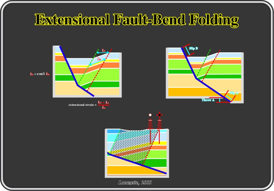
Fig.158- Folding requires extensional strain. Stratigraphic length L1 must extend to length L2 in the folded panel. The Coulomb shear model makes specific, quantitative predictions about rock strain. Good quality seismic data often resolves the fault and bedding orientations well enough to predict the amount of strain in the folded panel. Regardless of whether or not strain can be computed from seismic data, fold panels of this type must be areas of extensional strain. Slip and throw change across the fault bend. The Coulomb shear model makes specific, quantitative predictions about relative slip magnitudes/rates, and subsidence amounts/rates for each fault segment. In this example, the slip on segment B is 15% greater than the slip on segment A and stratigraphic throw across segment B is 88% greater than across segment A. Consequently, during fault movement the slip rate must have been correspondingly faster on segment B than was the subsidence rate above segment B. The variations in slip rate/amount may be an important control on the size and damage intensity of the fault damage zone. If folding-related strain is accommodated by brittle fracturing, then we can predict where fractures are developed with simple structural models.

Fig. 159- Faults also develop steepening bends. Deformation at a steepening bend can be treated with the same Coulomb shear model and equations previously discussed for flattening bends. In this case slip along segment A appears to require the hangingwall block above segment B to penetrate the footwall block, which is impossible if material is conserved. Both extension and shortening are geometrically acceptable solutions to the space problem. However, only extensional folding is compatible with extensional stress because shortening requires the wrong shear-sense at the active axial plane. Folding of the type depicted in the bottom right sketch (Shortening) indicates wrench faulting and/or polyphase deformation.

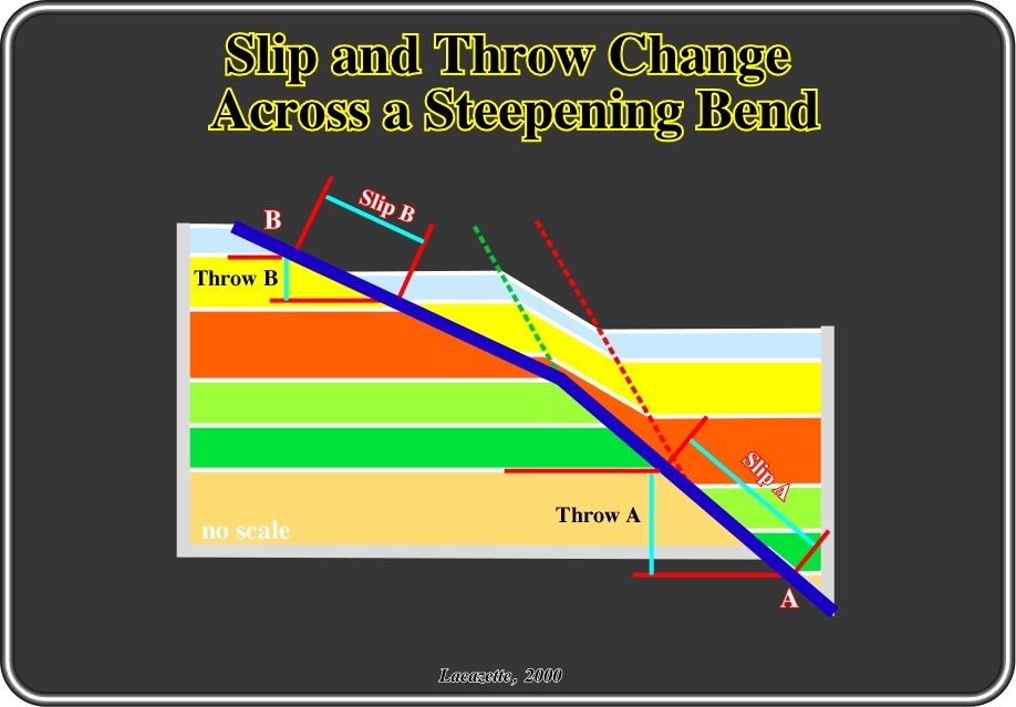
Fig. 160- As in the case of a flattening bend, the Coulomb shear model makes specific, quantitative predictions about relative slip magnitudes/rates, and subsidence amounts/rates for each fault segment. Again, both fault slip and stratigraphic throw change across the fault bend. In this example, the slip on segment B is 68% of the slip on segment A and stratigraphic throw across segment B is 45% of that across segment A. During fault movement, the slip rate is correspondingly slower on segment B as is the subsidence rate above segment B. Again, the variations in slip rate/amount may be an important control on the size and damage intensity of the fault damage zone. Steepening and flattening bends may appear to be simple geometric opposites of each other, but there is a critical difference: At at steepening bends the friction on the upper fault segment is higher than on the lower fault segment but the reverse is true on a flattening bend. Because of this difference, the hangingwall above a steepening bend tends to detach causing the fault to steepen or straighten but the hangingwall above a flattening bend tends to move with the rest of the block and undergo extensional folding as it collapses to fill the void.

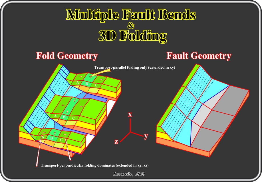
Fig. 161- This figure illustrates two important complexities that all real faults exhibit: Multiple fault bends and fault bends parallel to the transport direction. The hangingwall of a fault with multiple bends can experience multiple distinct episodes of deformation in a single continuous deformation, as shown in the previous figure. Fold panels A and C are folded about an axis perpendicular to the transport direction, but A and C are strained by different amounts because the angles of the transport-perpendicular fault bends that produce each panel are different. All three fold panels are folded about an axis parallel to the transport direction, but fold panel B suffers transport-parallel folding only. As a package of rock passes from A to B deformation changes from a combination of transport-perpendicular and transport-parallel folding to transport-parallel folding only. Rocks passing from B to C also undergo a second deformation. The hangingwall block shown in Fig.155 will contain at least 12 distinct structural domains. The number of folded panels is doubled because the left and right sides of the hangingwall block are mirror images of each other. Thus, the orientations of the strains are different which causes the fractures on each side to have different orientations. Initial and final refer to the periods before and after enough extension occurs for rocks from panel A to become part of panel C. Quantitative structural analysis can divide geologic structures into domains with homogeneous deformational histories. Quantitative fracture data at one location in a domain can be extrapolated throughout the domain, so that a fracture model for an entire field can be estimated in three dimensions.