Porto, Portugal
Contents:
1.1) Definitions
       1.1.1- Mechanical Field
       1.1.2- Forces
                 1.1.2.1- Forces acting in a Body
                 1.1.2.2- Forces acting on a Surface
       1.1.3- Stress
       1.1.4- Displacement
       1.1.5- Strain
       1.1.6- Rheological Laws
       1.1.7- Stress Vectors
       1.1.8- Stress Components
                 1.1.8.1- Normal Component
                 1.1.8.2- Shearing or Tangential Component
       1.1.9- Stress Tensor
1.2) Stress Ellipsoids
       1.2.1- Principal Axes
       1.2.2- Types of Stress Ellipsoids
                 1.2.2.1- Anisotropic Stresses
                              1.2.2.1.1- Triaxial
                               1.2.2.1.2- Biaxial
                 1.2.2.2- Isotropic Stress or Hydrostati
1.3) Stresses in Rocks
       1.3.1- Geostatic Pressur
       1.3.2- Pore Pressure
       1.3.3- Tectonic Pressure
       1.3.4- Effective Stresse
1.4) Tectonic Stress & Stress Field
       1.4.1- Horizontal Extension
       1.4.2- Horizontal Compression
1.5) Rheology & Experiment Laws
       1.5.1- Definitions
                 1.5.1.1- Elastic Material (Hookean solid)
                 1.5.1.2- Viscous Material (Newtonian liquid)
                 1.5.1.3- Plastic Material
                 1.5.1.4- Ductile Material
                 1.5.1.5- Brittle or Rigid Material
                 1.5.1.6- Fluid
       1.5.2- Mechanical Behaviors of Rocks
                 1.5.2.1- Mechanical Analogue Conditions
                 1.5.2.2- Experimental Conditions
1.6) Deformations
       1.6.1- Deformation with Failure
                 1.6.1.1- Mohr’s Theory
                 1.6.1.2- Mohr’s Circle
                 1.6.1.3- Mohr’s Envelope
                 1.6.1.4- F Evolution with Increasing Stresses
                 1.6.1.5- Pore Pressure and Rupture
                 1.6.1.6- Pre-fractured Rock
                 1.6.2- Deformation without Failure
1.1.1- MECHANICAL FIELD
At a given time, for a particular system, the mechanical field is characterized by:
a) The position and the velocity of each part composing the system, and
b) The stresses acting in the different parts of the system.
The differences between two mechanical fields are generally described by:
(i) Displacement.
(ii) Deformation.
(iii) Stress Fields.
1.1.2- TYPES OF FORCES
Forces can be subdivided into two types:
1.1.2.1- Forces acting in a Body
The force acts in all material composing the body. Its value is proportional to the mass of the body. Ex: Gravitational Force, Centrifuge Force, Magnetic Force, etc.
1.1.2.2- Forces acting on a Surface
These forces act on the surface of a body. Generally, they are measured by the value of the force divided by the surface in which they act.
1.1.3- STRESS
In any grain of a rock there is a force, which can be transmitted by nearby grains or by the fluid containing in the porosity. In a rock, stress is the force per unit area, acting on any surface within it, and variously expressed as pound or tons per square inch, or dynes or kilograms per square centimetre. By extension, stress represents the external pressure, which creates the interval force.
1.1.4- DISPLACEMENT
The displacement is described as the position change of a particle or a body.
1.1.5- DEFORMATION
Deformation is the expression of the percentage of configuration change, for instance the longitude of a line in relation to its initial longitude. Deformation compares two conditions at two different times.
Deformation relates the initial instantaneous configuration, which usually is taken as initial condition, or initial state, without deformation, with a posterior configuration. The same idea of initial condition can be applied to displacement.
1.1.6- RHEOLOGICAL LAWS
Are the laws expressing the relations between stress and deformation.
1.1.7- STRESS VECTOR
Stress vector describes the state of stresses in a plane inside a rock.
1.1.8- STRESS COMPONENTS
The stress at a given point is mathematically defined by nine values:
- Three to specify the normal components.
- Six to specify the shear components, relatively to three mutually perpendicular reference axes.
Stress is a tensor of second rank. The forces area thought to act on every one of the infinitesimal elements of area with different orientation, which can be imagined at one point. Only such forces are considered, which are locally in equilibrium with equal and opposite forces: Tensor is symmetrical. The stress across a plane through any given point located at the surface or inside of a rock can be resolved into two components:
a) Normal stress, symbolized by Greek letter
, acting normal to the plane.
b) Shearing stress, or tangential stress, symbolized by Greek letter t, acting along the plane, perpendicular to the normal stress.
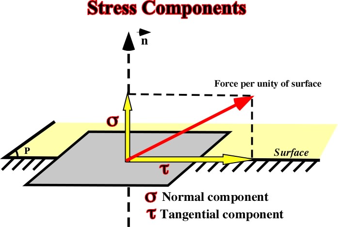
Fig. 1- Normal and shearing components of a stress applied on a surface.
Normal stresses can be:
a) Compressional or Positive
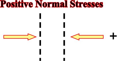
Fig. 2- Compressional or positive normal stresses are generally depicted by convergent arrows or by a symbol plus.
b) Tensional or Negative
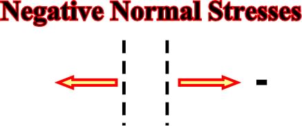
Fig. 3- Tensional or negative normal stresses, acting in a plane, are represented by two arrows in opposite directions or by the symbol minus.
Shearing or Tangential stresses can be:
a) Dextral or Clockwise
They are dextral when the upper side of the surface is sheared to the right, that is to say, in the direction to that in which the hands of a clock rotate as viewed from in front.
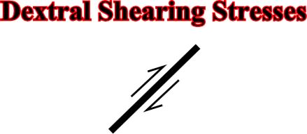
Fig. 4- Very often, dextral shearing stresses are represented, as dextral fault, by two opposite arrows, one above and the other below the plane, indicating that the upper part is displaced to the right.
b) Sinistral or Counterclockwise
They are sinistral or counterclockwise when the upper side of the surface is sheared to the left, that is to say, in opposite direction to that in which the hands of a clock rotate as viewed from in front.
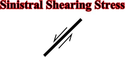
Fig. 5- Sinistral shearing stresses are represented, as sinistral fault, by two opposite arrows, one above and the other below the plane, indicating that the upper part is displaced to the left.
1.1.9) STRESS TENSOR
Stress tensor is a collection of stress for planes of all possible orientation. At one point, it is described by a stress tensor of second order. The surface forces applied to a geologic body can be solved in three Cartesian coordinate axes (stress ellipsoid). In a given point, the stress field is represented by nine components referred to three orthogonal coordinate axes:
- Three of the components are normal stresses acting perpendicularly to the coordinate planes.
- The other six components are shearing stresses or tangential acting along the coordinate planes.
Stress tensor can be represented by a mathematical formula, in which the Eigen vectors of the tensor (![]() ) corresponds to a matrix.
) corresponds to a matrix.
Supposing a body (![]() ) with an arbitrary point M (located inside or on the surface of the body). The given point M can be defined by three orthogonal coordinates:
) with an arbitrary point M (located inside or on the surface of the body). The given point M can be defined by three orthogonal coordinates:
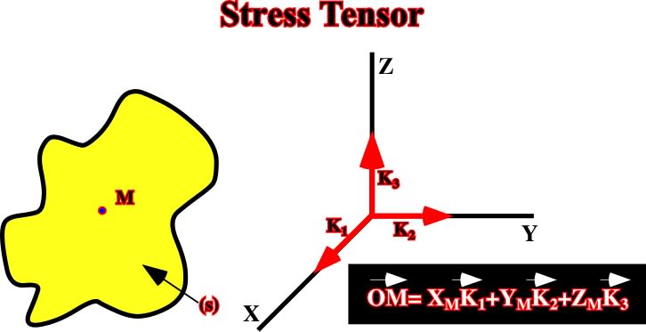
Fig. 6- The arbitrary point M can be defined by three orthogonal coordinates, where K1, K2 and K3 are unitary vectors.
The body (s) is submitted to the influence of body and surface stresses. For all point M, there are contact actions, which define a stress field. Taking an imaginary plane (P) passing through M, the plane P can be defined by the orthogonal vector n (n1, n2, n3) (fig. 7 & 8).
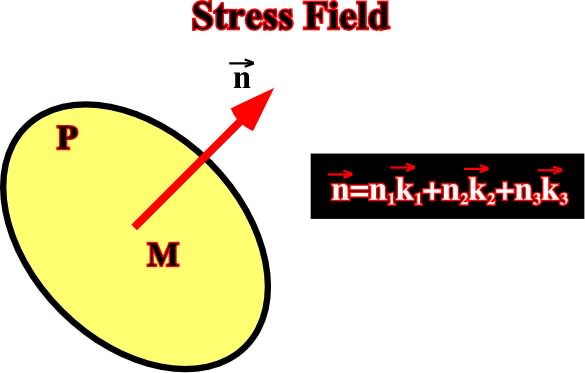
Fig. 7- The stress field for the point M is defined by the vector T= (M,n), see fig. 8.
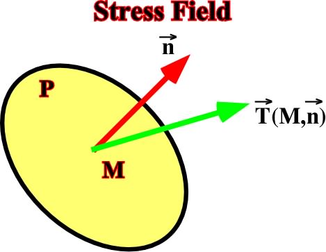
Fig. 8 - The stress vector (T) can be represented by three components T=(M,n), and (M+n) = T1 k1 + T2 k2 + T3 k3.
The relations between (T1,T2,T3) and (n1, n2, n3) are:
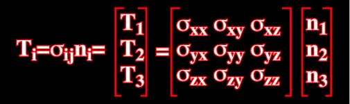
The nine ![]() ij are stress components for the given point M, defined in relation to three coordinates planes (ox,oy), (oy,oz) and (oz,ox), and
ij are stress components for the given point M, defined in relation to three coordinates planes (ox,oy), (oy,oz) and (oz,ox), and ![]() ij is a tensor.
ij is a tensor.
The stress component ![]() ij, by definition, is defined by the local normal vectors, within the reference system (o, k1,k2,k3). The nine stress components can be represented graphically as illustrated below (fig. 9).
ij, by definition, is defined by the local normal vectors, within the reference system (o, k1,k2,k3). The nine stress components can be represented graphically as illustrated below (fig. 9).
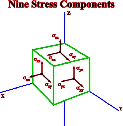
Fig. 9- Stress components can be illustrated graphically. All elements, that is to say, vector, point, body, etc., are referred to the coordinate axes (x,y,z), which origin is O.
Changing the coordinate system by a system having as origin the point M, the axis Z as N and the axes X and y on the plane P, the vector T can be decomposed into two vectors components Tn and Tt (fig. 10).
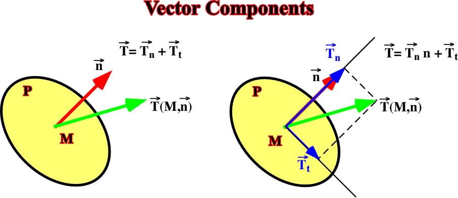
Fig. 10- In this figure, Tn is the normal stress and Tt the tangential or shearing stress. Conventionally, when Tn is positive, normally, there is compression, when Tn is negative there is extension.
The following assumptions must be made:
a) All these relations are related to the point M.
b) In a homogeneous stress field, the tensor
When the body (s) is in equilibrium, the fundamental equilibrium equation:
sF = m d = 0 (Newton)
is satisfied and the momentum of the stress F, in relation to the point O, is nil. The equilibrium equation gives:
![]() xy =
xy = ![]() yx
yx
![]() yz =
yz = ![]() zy
zy
![]() zx =
zx = ![]() x
x
Therefore ![]() is a symmetric tensor of the new tensors components. Only six tensors components are independent.
is a symmetric tensor of the new tensors components. Only six tensors components are independent.
The previous relationships are just for a particular direction, that is to say (n). However, rotating the vector (n) in all directions and taking the longitude Tn=0 it is possible to demonstrate that in an homogeneous and continuous medium, P will describe an ellipsoid (E), as illustrated in fig. 11.
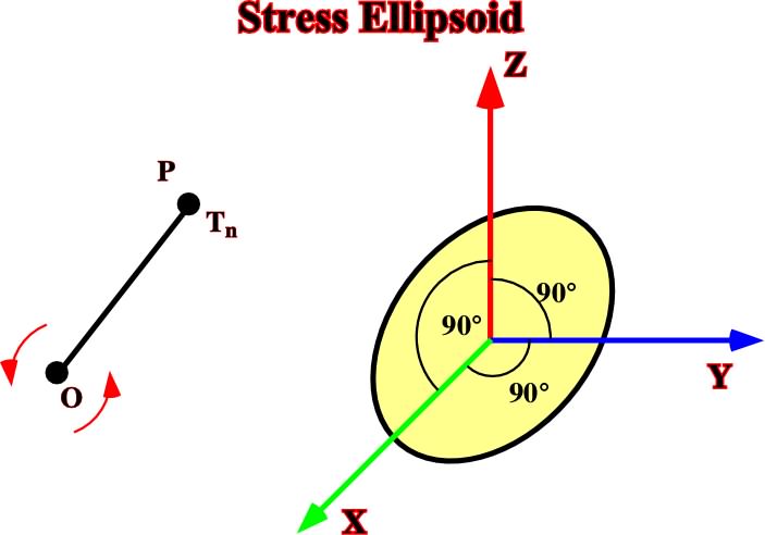
Fig. 11- Stress ellipsoid creating by rotation of vector (n) in all direction. Such ellipsoid is characterized by the following equation:
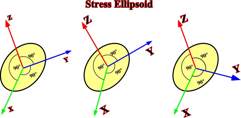
Fig. 12- Changing of coordinates does change the stress ellipsoid.
1.2.1) Principal axes
Among all coordinate systems only one satisfy the following condition:
![]() xy =
xy = ![]() yx =
yx = ![]() zx = 0
zx = 0
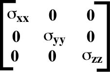
The three axes of that system are named the principal axes of the stress ellipsoid (E), along which there are no tangential or shearing stresses. The tensor is:
1.2.2) Types of Stress EllipsoidsTwo types of stress ellipsoids can describe the stress conditions within earth’s crust:
1.2.2.1- Anisotropic ellipsoids
Assuming homogeneous and continuous rocks, two anisotropic ellipsoid are possible:
1.2.2.1.1- Triaxial (fig.13)
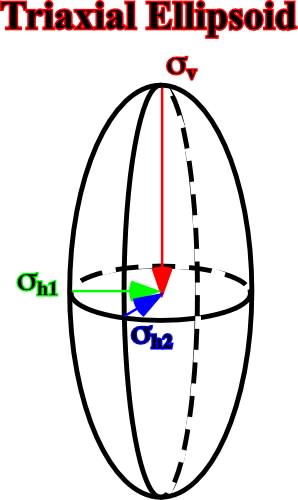
Fig. 13- In a triaxial ellipsoid, the three principal axes are different.
A triaxial ellipsoid, as well as others ellipsoids, can be simplified in a bi-dimensional graphic, that is to say, whether by a Mohr’s circle (fig. 14) or by a Mohr’s envelope (fig. 52).
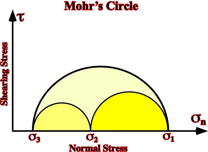
Fig. 14- The Mohr’s circle is a graphic representation of the state of stress at a given point at a given time. The coordinates of each point on the circle are the shear stress and the normal stress on the given plane. The Mohr envelope (fig. 52) is an envelope of a series of Mohr circles, that is to say, the locus of points whose coordinates represent the stresses at failure.
1.2.2.1.2- Biaxial (Fig. 15)
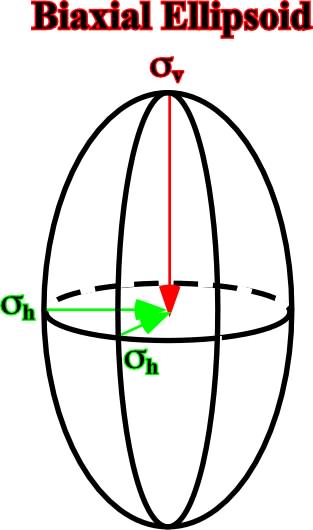
Fig. 15- In a biaxial ellipsoid there are only two principal axes. The vertical axis (
1.2.2.1.3- Isotropic ellipsoids
The isotropic or hydrostatic ellipsoids are uniaxial, that is to say, that they have just one axis, as a sphere (fig. 16).
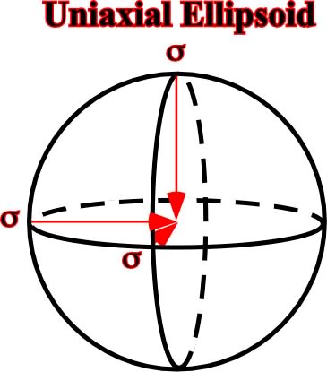
Fig. 16- In an uniaxial ellipsoid the stress stays constant independently of its orientation. The ellipsoid has the shape of a circle and its radius is
The field of states of stress, homogeneous or varying from point to point and through time in a given defined domain, is called stress field. At depth, the state of stress in rocks, at a given point, is the result of three factors: (1.3.1) Geostatic or Lithostatic stress; (1.3.2) Pore pressure; (1.3.3) Tectonic stress; (1.3.4) Effective Stresses.
1.3.1) Geostatic or Lithostatic stress (
At a given depth, the geostatic stress (
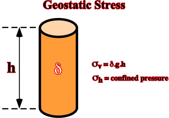
Fig. 17- The hydrostatic stress can be depicted by a biaxial ellipsoid, in which the sv is the weight of the sedimentary column (d.h.g) and the
Assuming a sedimentary basin with undeformed homogeneous and continuous rocks, the stress field is characterized by a biaxial ellipsoid. However, the geostatic stress ellipsoid varies with depth. The state of stress tends to become hydrostatic at great depth (fig. 18):
- Near the surface, rocks of a elastic behavior, therefore:
- At medium depth, rocks of a viscous-elastic behavior, therefore: 1/3
- At great depth, rocks of a viscous behaviour, therefore:
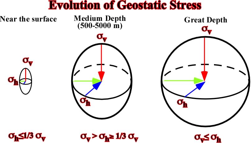
Fig. 18- This figure illustrates the evolution in depth of the geostatic stress. Near the surface, the ellipsoid is biaxial and oblong, but in depth becomes almost uniaxial. Such a feature explains, partially, why fault planes flatten in depth.
1.3.2) Pore Pressure or Hydrostatic stress (
The pore pressure sp is the pressure of the interstitial fluids. In geology, the fluids generally water, saturating the open pore spaces of a rock column produce a tantamount effect as immersing a rock in a water column (fig. 19):
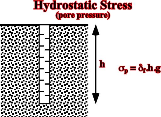
Fig. 19- At a given depth, the pore pressure can be represented by a uniaxial ellipsoid, that is to say, a sphere, which radius is the product of the density of the fluid (df). The depth of the given point is (h) and the gravitational force is (g).
When a porous body is enclosed within an impermeable environment, its interstitial fluid does not communicate with surface, therefore it is not any more in a purely hydrostatic condition but in an overpressured state. The overpressures are normally due to:
a) The rapid burial of rocks with low permeability (shales, evaporites).
b) The temperature in closed systems.
c) The changes in tectonic phases.Since these conditions produce: (1) abnormal porosities and (2) low densities. The overpressures can explain:
(i) Growth faulting.
(ii) Under-compacted shales.
(iii) Mud volcanoes.
(iv) Slumping.
(v) Tectonic soles and over-thrusts.Interstitial pore pressures act on the grains of a rock in opposite direction of the lithostatic and tectonic stresses (fig. 20).
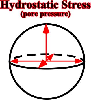
Fig. 20- Pore or hydrostatic pressure acts in opposite direction of the lithostatic pressure. It explains buoyancy, that is to say, the upward thrust on a body immersed in a fluid. This force is equal to the weight of the fluid displaced (Archimedes’ Principle).
As pore pressure (
A) In normal conditions
In an open water system all pores are in communication. In absence of tectonic stress, the depth evolution of pore pressure (
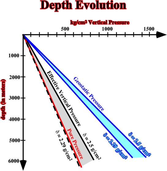
Fig. 21- This cross-plot represents the evolution, in depth, of the geostatic pressure, pore pressure and effective vertical pressure.
B) In Overpressure conditions
In absence of tectonic stresses, the presence of overpressure zones reduces the effective vertical pressure, as illustrated in fig. 22, in which are represented the evolution, in depth, of: (a) Pore Pressure, (b) Geostatic Pressure, (c) Vertical Effective Pressure, (d) Transition Zone and (e) Top of Overpressure Zone.
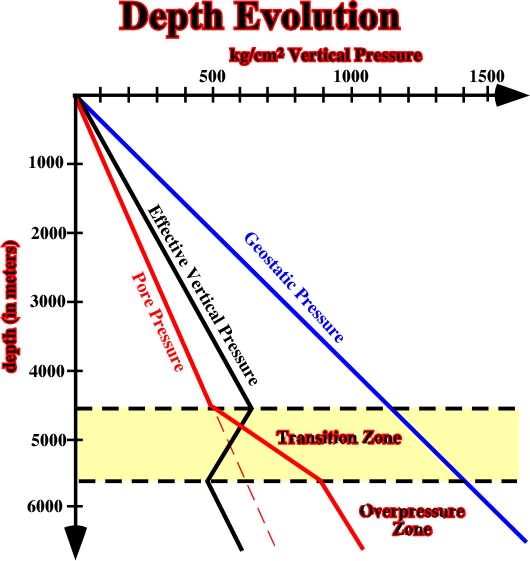
Fig. 22- This cross-plot illustrates the evolution, in depth, of vertical effective pressure in a basin with an overpressure zone.
1.3.3) Tectonic Stress (
Tectonic stress (
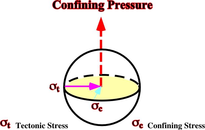
Fig. 23- When a tectonic stress is added in a given direction, it induces, by reaction, a lateral confined pressure. Upward (free surface) an equilibrium pressure is created whether by uplift or subsidence.
1.3.4) Effective Stress (
The effective stress is the result of the geostatic stress (
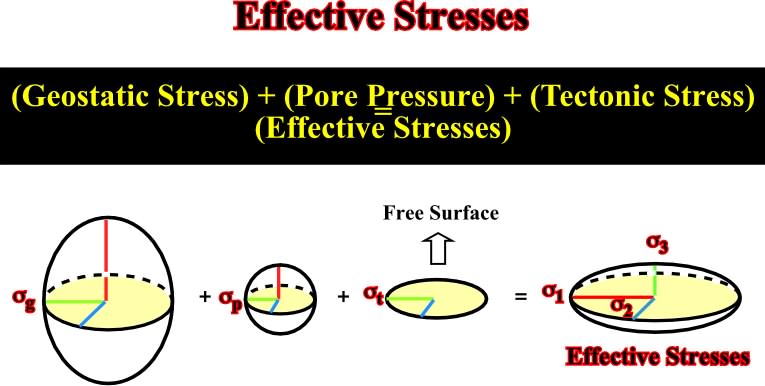
Fig. 24- The effective stresses (
Conventionally:
A) When
B) When
1.4- Tectonic Stress & Stress Field
The consequences of the tectonic stress in a stress field, can be roughly recognized by adding to an initial state of stresses increments of tectonic stress, whether positive (compression) or negative (extensional tectonic stress). The following numerical example is not completely correct, but it can help us to understand how and why rocks are deformed.
Let’s start to assume, homogeneous and continuous rocks with an undeformed planar surface, at a middle depth. In addition, let’s assume, that (i) the rocks have a viscous-elastic behavior and (ii) the confining pressure is roughly 8/10 of the geostatic pressure (![]() h = 8/10
h = 8/10 ![]() g). At a given point at 3000 meters depth, with an average sedimentary density of 2.5 g/cm3 and with an interstitial fluid density of 1.1 g/cm3 (water), we can calculate:
g). At a given point at 3000 meters depth, with an average sedimentary density of 2.5 g/cm3 and with an interstitial fluid density of 1.1 g/cm3 (water), we can calculate:
The Initial State of Stresses
a) Geostatic Pressure
The geostatic pressure is given by a biaxial ellipsoid (fig. 25), with
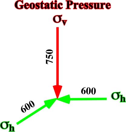
Fig. 25- Principal axes of the ellipsoid representing the geostatic pressure ![]() g.
g.
b) Hydrostatic Pressure
The hydrostatic pressure is given by a uniaxial ellipsoid (fig. 26), with
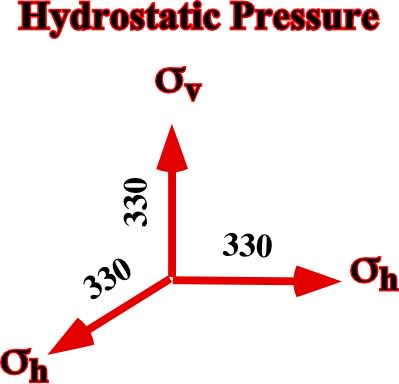
Fig. 26- Principal axes of the ellipsoid representing the hydrostatic pressure ![]() p.
p.
c) Effective Vertical Pressure
The effective vertical pressure is given by the geostatic pressure minus the hydrostatic pressure, that is to say that it corresponds to a biaxial ellipsoid (fig. 27), with
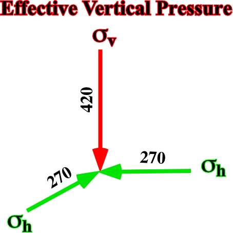
Fig. 27- Principal axes of the ellipsoid representing the effective vertical pressure ![]() ev.
ev.
Knowing the effective vertical pressure one can now add the tectonic stress.
Let’s start adding: a negative tectonic stress (
1.4.1- Horizontal Extension
a) Adding a tectonic stress of -100kg /cm2 along the axis Y, we get a tridimensional ellipsoid (fig. 28) with:
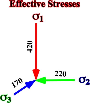
Fig. 28- Principal axes of the ellipsoid of effective stresses after adding a tectonic stress of -100 kg/cm2 (horizontal tension) along the axis Y (blue) of a bidimensional vertical effective stress with
b) Adding a tectonic stress of -200kg /cm2 along the axis Y, we get a tridimensional ellipsoid (fig. 29) with:
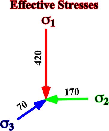
Fig. 29- Principal axes of the ellipsoid of effective stresses after adding a tectonic stress of -200 kg/cm2 (horizontal tension) along the axis Y of a bi-dimensional vertical effective stress with
c) Adding a tectonic stress of -400kg/cm2 along the axis Y, we get a tri-dimensional ellipsoid (fig. 30) with:
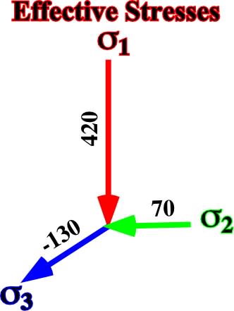
Fig. 30- Principal axes of the ellipsoid of effective stresses after adding a tectonic stress of -400 kg/cm2 (horizontal tension) along the axis Y of a bi-dimensional vertical effective stress with
It is relevant to point out that in all previous examples there is no change or rotation of the main axis of the effective stress ellipsoid, only their value changes.
Now, let’s add, along the same axis (Y), a positive or compressive tectonic stresses.
1.4.2- Horizontal Compression
a) Adding a tectonic stress of 100kg /cm2 along the axis Y, we get a tridimensional ellipsoid (fig. 31) with:
Fig. 31- Principal axes of the ellipsoid of effective stresses after adding a tectonic stress of 100 kg/cm2 (horizontal compression) along the axis Y of a bidimensional vertical effective stress with
b) Adding a tectonic stress of 200kg /cm2 along the axis Y, we get a tridimensional ellipsoid (fig. 32) with:
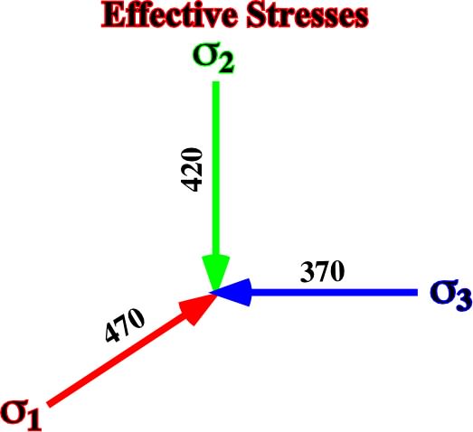
Fig. 32- Principal axes of the ellipsoid of effective stresses after adding a tectonic stress of 200 kg/cm2 (horizontal compression) along the axis Y of a bidimensional vertical effective stress with
c) Adding a tectonic stress of 400kg /cm2 along the axis Y, we get a tridimensional ellipsoid (fig. 33) with:
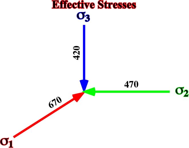
Fig. 33- Principal axes of the ellipsoid of effective stresses after adding a tectonic stress of 400 kg/cm2 (horizontal compression) along the axis Y of a bidimensional vertical effective stress with
It is interesting to note than the effective stresses (
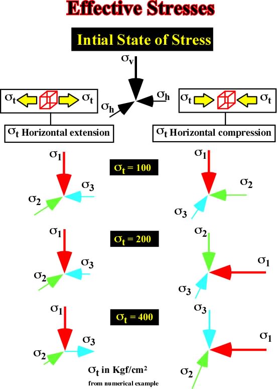
Fig. 34- This sketch summarize all possible ellipsoids of effective stresses (
1.5- Rheology & Experiment Laws
1.5.1- Definitions
In the crust of the earth, the ellipsoid of effective stresses changes during geological time. The effective stresses induce permanent deformations in the sediments. One of the targets of Structural Geology is to determine the nature and the amplitude of the sedimentary displacements. Geologists can determine the sequence and the amount of deformation in a zone under effective stresses. It is theoretically possible to relate the sedimentary deformations to the effective stresses producing them. In other words, geologists observing the geometry of the deformed sediments can deduct the ellipsoid of effective stresses. The relationships between stress and strain (deformation) are useful to describe the behavior of rocks on a macroscopic scale. At this scale, the rocks can be described as continua so that the in-homogeneities and anisotropies associated with their polycrystalline nature are averaged out. However, the relationship between stress and strain depends on the rheology of the sediments, which is expressed by laws and few simple mathematical idealizations (constitutive equations) of the material behavior.
Different materials behave differently under the same stress. For example, under a uniaxial compression, one type of material might shorten slightly and then stabilize, whereas another might flow continuously like putty. From experiments we can observe the different types of mechanical behavior in rock and how each depends on (i) stress, (ii) temperature, (iii) pressure, (iv) grain-size, (v) composition and (vi) chemical-environment. Continuum models of material behavior can be summarized as follow:
1.5.1.1- Elastic Material (Hookean solid)
When a material is subjected to stress it deforms. The material is said to be perfectly elastic if, when stress is removed, the deformation completely and instantly disappear (deformation is said recoverable).
The theory of elasticity most commonly used is based upon for simplifying assumptions, namely that the elastic material is:
(i) Homogeneous,
(ii) Isotropic, and that(a) Elastic strains are infinitesimal (extremely small) as well as
(b) Stress-strain relationships.So a body is said elastic when strains are instantly and totally recoverable and in which deformation is independent of time. The stress strain relationship is represented by a linear equation, which states either a normal stress
ts= 2m es
The constant E is Young’s modulus and m is the shear modulus or the modulus of rigidity (fig. 35).
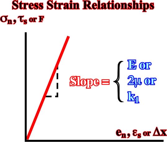
Fig. 35- The stress-strain relationships in a linear elastic (Hookean) solid (or a spring) are here illustrated by a plot of normal stress (or force) versus extension, where the slope E (or k1) is the Young’s modulus (or spring constant).
These equations are identical in form to Hooke’s law (1660), which describes the behavior of a spring (see later).
1.5.1.2- Viscous Material (Newtonian liquid)
At room temperature and pressure, a rock clearly reacts to stress very different from a material such as water. We cannot expect, therefore, that an equation for elastic behavior, which applies very well to cold rocks, would be very successful in accounting for the behavior of water.
If a stress is applied to a fluid, it begins to flow. When the stress is removed, the flow stops, but the fluid does not return to its undeformed configuration, and the deformation is said to be non-recoverable. The larger the applied stress, the faster the fluid flows, which suggests a relationship between the stress and the strain rate. This type of behavior is most simply idealized as a linearly viscous, or Newtonian, constitutive equation, and the appropriate one-dimensional equation for constant-volume deformation relates the normal deviatoric stress delta
delta
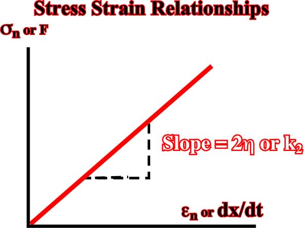
ts = 2h es
Fig. 36- The characteristics of a linear viscous fluid (or Newtonian) are here illustrated by the plot of stress (or force) versus incremental strain rate (or displacement rate). This plot has a slope h (or k2, dashpot)), that is to say the coefficient of viscosity (dashpot constant k2, see later).The incremental extension rate is the rate of change in length divided by the instantaneous deformed length. The incremental shear strain rate is half the rate at which the tangent of the incremental shear angle changes, where the incremental shear angle is measured for material lines instantaneously normal to one another. These strain rates are nothing more than strains defined by the incremental strain ellipse divided by the increment of time. The proportionality constant k is called the coefficient of viscosity of the fluid.
Liquid giving rise to linear relationships are known as Newtonian liquids, while those exhibiting a non-linear relationship are non-Newtonian.
1.5.1.3- Plastic Material
Under many conditions, including common experimental conditions in the laboratory, the model of the linearly viscous fluid does not describe well the observed behavior of polycrystalline solids, such as rocks and metals.
Such materials commonly undergo no permanent deformation if the applied stress is smaller than a characteristic yield stress, but they flow readily if it is at or slightly above the yield stress. Materials exhibiting this type of behavior are plastic materials.We idealize plastic behavior mathematically by assuming that there is no deformation at all (the material is rigid) below the yield stress and that during the deformation, the stress cannot rise above the yield stress except during acceleration of the deformation. This model describes a perfectly plastic material or a rigid-plastic material.
The stress for ductile flow is a constant and the constitutive equation is the von Mises yield criterion:
|

Fig. 37- This figure illustrates the characteristics of a perfectly plastic (Saint Venant) material on a plot of stress (or force) versus incremental strain rate (or velocity).
1.5.1.4- Ductile Material
Said of a body that is able to sustain, under a given set of conditions, 5 to 10% deformation before fracturing or faulting. Intense ductile deformation of rock usually takes place at:
(i) Considerable depth in the Earth’s crust where the temperature and confining pressures are high.
(ii) Before the sediments have been completely indurate.
By the time that rocks are studied by geologists, they are usually at, or near, the surface, so that intensely deformed rocks have passed through an environment of relatively low temperature and confining pressure. If, for instance, fractures develop in both the prograde and retrograde deformation environments it follows that the more ductile type of fractures will pre-date the brittle type of structure. (NB- We used the terms relating to deformation in the way they relate to metamorphism: prograde deformation is associated with downward and /or orogenesis and retrograde deformation occurs in the phase of uplift and exhumation).
1.5.1.5- Brittle or Rigid Material
Said of a material that fractures at less than 3-5% deformation or strain. When tested to failure under conditions of triaxial compression, many competent rocks exhibit a relationship between principal stresses at failure, which is represented by the empirically derived linear equation:
Where
However, other rock types exhibit a non-linear relationship between principal stresses at failure. In these types of tests the specimens fail in shear. Usually the specimens fail along only one shear plane. Occasionally specimens exhibit two conjugated shear planes, with opposite shear sense. The angle between them, which is often considerably less than 90°, is bisected by the axis of maximum principal stress.
1.5.1.6- Fluid Material
Said of a material that when deformed does not have an instantaneous and totally recuperation of its initial state, without loss of coherence. A perfect fluid offers no resistance to change of shape (i.e. has zero viscosity).
The rheologic models are largely insufficient to take into account all cases occur in earth’s surface. The Rheological laws must take into account the different possible scales, as for instance: time (1s, 1h, 1 year, 106 years, etc.), length (100 A°, 1 mm, 1m, 1km, 100km, etc.), temperature, pressure, etc..
Crustal materials have mechanical behaviors between two extreme cases:
- Fluid, when they have small and finite deformation under hydrostatic pressure.
- Solid, when they have finite deformation under tangential or hydrostatic stresses.
On the other hand, rheologic laws are dependent of:
- Effective stresses.
- Duration of the stresses.
- Temperature and Pressure.So, at atmospheric pressure (roughly 1 kg cm2) and at 25°C, a rock can have an elastic behavior. However, at 500 At of pressure and 250°C, it behaviors as plastic. In order to determine the mechanical behavior of a rock, one needs to know:
- The Stress Field (tensor).
- The Strain Field (tensor).
- The Stress - Strain ratio (Rheological Law).The mechanical behavior can be approach whether by mechanical analog or under experimental conditions.
1.5.2- Mechanical Behaviors of Rocks
1.5.2.1- Mechanical Analogs
A) Solid
a) Ideal Solid (Euclides)
No deformation in spite of large stress.
b) Hooke’s solid (linear elasticity)
The mechanical analogue to elastic behavior (see 1.5.1.1, fig. 35) is a spring (fig. 38). Strain is proportional to stress (fig. 35).
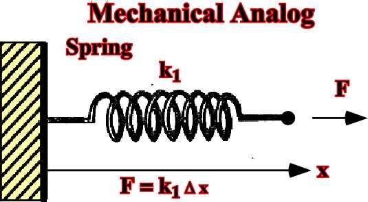
Fig. 38- A mechanical analogue to elastic behavior (strain is proportional to stress) consists of a spring with spring constant k1 attached to a rigid wall, subjected t a force F, and displaced a distance Dx beyond its unloaded length.
c) Plastic solid (Saint Venant)
The mechanical analogue to plastic flow (see 1.5.1.3, fig.37) is the frictional resistance to sliding of a block on a plane (fig. 39).
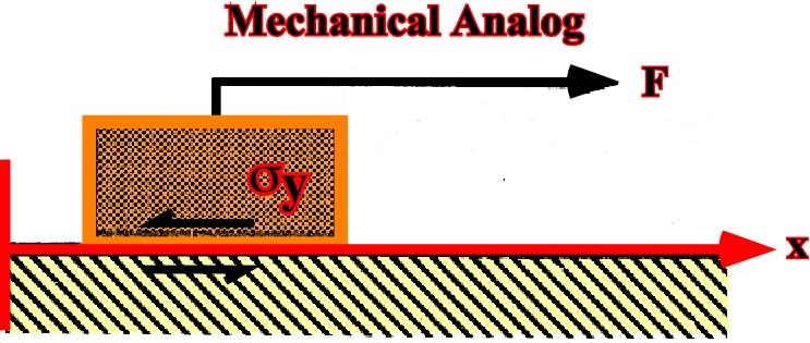
Fig. 39- A plastic solid behavior (strain starts when shearing exceeds a threshold) can be depicted by a body over a planar surface displaced by a rope. Once sliding has started, the applied force cannot rise above the frictional resistance regardless of the velocity of sliding, except during acceleration. Thus the force history produces an undefined rate of displacement.
B) Liquid
a) Pascal liquid incompressible and b) Newtonian liquid
A mechanical analogue for viscous behavior (see 1.5.1.2, fig. 36) is a dashpot or absorbent shock (fig. 40), since the stress is proportional at the rate of deformation.
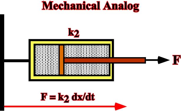
Fig. 40- The analog of viscous behavior (Newton liquid) is tin a dashpot consisting of a porous piston in a cylinder containing a viscous fluid, attached to a rigid support, and subjected to a force F.
Actually, when a force is applied across the system, the motion of the piston is governed by the rate at which fluid can flow through the pores in the piston.The greater the applied force, the faster the piston moves A force suddenly applied to the dashpot at time t1 and suddenly removed at t2 produces a linear increase of displacement between those times, and it leaves a permanent displacement when the force is removed.
C) Complex Mechanical Behavior
The simple elastic, plastic and viscous models summarized previously do not describe adequately all-important material behavior. Complex model combining the simple models in series or in parallel can often better explain rock behavior
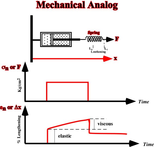
a) Viscous-Elastic (Maxwell) Solid
A visco-elastic solid (Maxwell) behaves like a combination in series of an elastic spring and a viscous dashpot (fig. 41). The permanent strain accumulates viscously, and it begins as soon as stress is applied.
For high viscosities, this material behaves like an elastic material for loads of short duration but like a viscous material for long-term loads.
For constant imposed strain, the initial elastic response is gradually converted into permanent viscous deformation, and the associated stress decays with time. Visco-elastic behavior resembles that of a silly putty. It is useful in modeling the response of the Earth’s crust, which is observed to undergo short-term elastic deformation when subjected to a rapid loading, but which gradually flows if the load is maintained for long periods.
Fig. 41- The characteristics of a visco-elastic, or Maxwell, material are here illustrated by a mechanical analogue consisting of a dashpot in series with a spring. The plot sn or F versus time shows the stress-time history imposed on the material, while the plot en or Dx indicates the natural strain-time response to the imposed stress, which includes an instantaneous recoverable elastic deformation and a non recoverable viscous deformation.
b) Elastic - Plastic (Prandtl)
This model corresponds to a Hooke solid and a plastic solid (fig. 42).
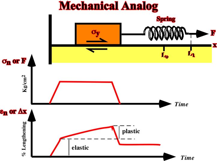
Fig. 42- The mechanical analogue for an elastico-plastic material (or Prandtl) consists of a friction block connected in a series with a spring. An imposed stress-time history and the corresponding natural strain-stress history are also illustrated. Below the yield stress, the material deforms elastically. At the yield stress, plastic deformation occurs at undetermined rate. When stress is removed, the elastic portion of the strain recovers, leaving a permanent strain equal to the plastic portion.
c) Viscous-plastic (Bingham)
A plastic solid and a Newtonian liquid can simulate a viscous-plasticmaterial (fig. 43). Such a model displays linear viscous behavior only above a yield stress (plastic materials).
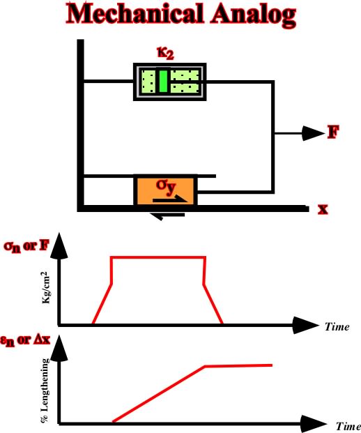
Fig. 43- Here are illustrated the characteristics of a visco-plastic, or Bingham material. The mechanical analogue consists of a dashpot and a friction block connected in parallel. A stress-time history and the subsequent natural-strain-time history resulting from the imposed stress are also depicted.
A natural example of this behavior is wet paint. It is a fluid but has a small yield stress, which prevents it from running off a wall after a thin layer is applied.
d) Firmo-viscous (Kelvin or Voigt)
A firmo-viscous material is elastic to the extent that the equilibrium strain is a linear function of the applied stress, but the strain rate is governed by a viscous response. An everyday application of the mechanical analogue is an automobile suspension system consisting of a spring connected in parallel with a dashpot (s shock absorber), which damps out elastic oscillation of the spring.
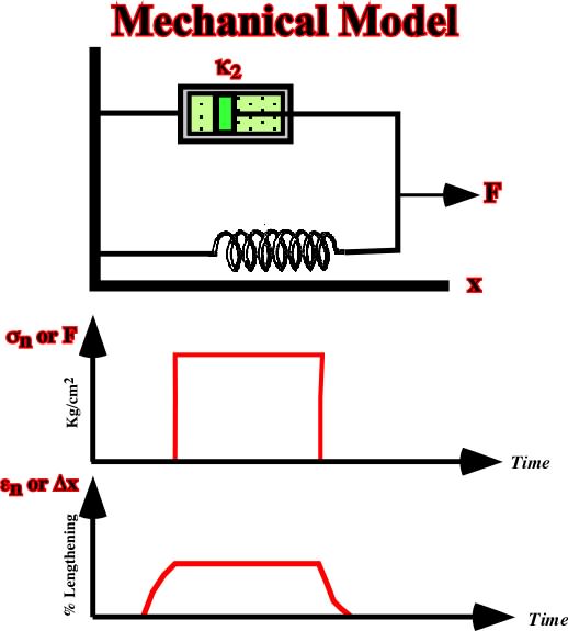
Fig. 44- The mechanical analogue of a firmo-viscous behavior consists of a dashpot and a spring connected in parallel as illustrated. The natural strain-time response of an imposed stress-time history shows that the incremental strain rate depends both on the initial stress and on the strain.
Combining the simple mechanical analogues in different combinations can derive other models. The potential usefulness of any such model depends on whether its response corresponds to that observed for a particular material. All these models, with the exception of plasticity, have the limitation that they are superposition of the linearly proportional responses of a spring or dashpot to an imposed load.
Such linear models have proved extremely useful in many applications in geology and engineering, but materials do not have to behave in mathematically convenient ways.
Thus nonlinear elasticity theory is necessary to account for the elastic properties of rocks under vary high pressures, and some of the processes of ductile flow crystalline solids are inherently nonlinear.
1.5.2.2- Under experimental conditions
The behavior of rock deformation under stresses, have been determined using triaxial detectors where the confining pressure is controlled during the application of triaxial stresses, either compression or tensional stresses. The stress-strain curbs are obtained to different (i) Temperatures, (ii) Confining pressures, (iii) Percentage of deformations and (iv) Rock-type (fig. 45). During the test different stages of deformation appear as:
(i) Elastic deformation.
(ii) Late fractures when the rock breaks instantaneously.
(iii) Permanent plastic deformation when the material is not brittle with acquisi-tion of permanent deformations.
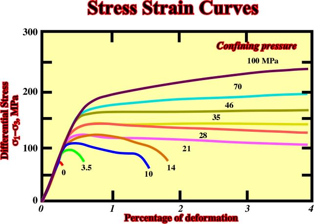
Fig. 45- Progression of stress-strain curves with increasing of confining pressure in the Wombeyan marble (from Paterson, 1978).
Figures 46 and 47 illustrate two examples of complex rheology.
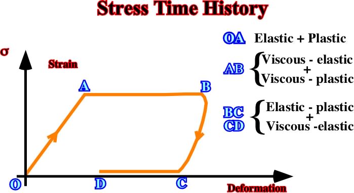
Fig. 46 –In this example, the stress-time history and the associated natural stress-time response are shown. The behavior is elastic-plastic during OA, then during AB it comes visco-elastic / viscous-plastic, and finally, between BC and CD it is Elastic-plastic / visco-elastic.
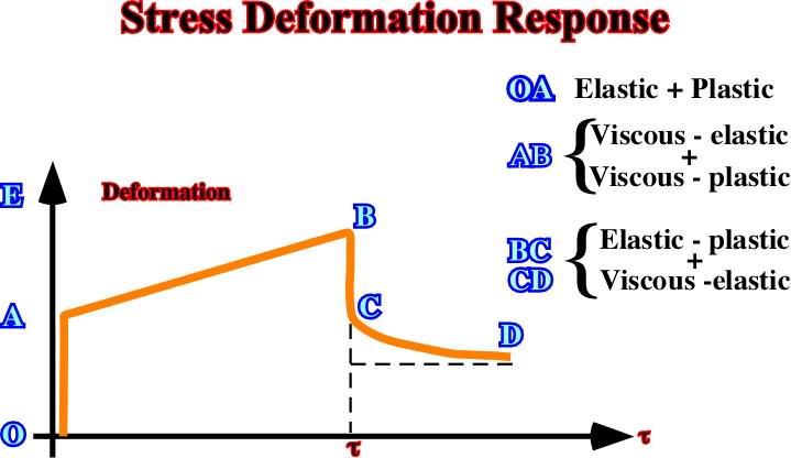
Fig. 47- In this stress-deformation response, during OA the material behavior is elastic-plastic, during AB it behaves as visco-elastic / visco-plastic, while from B to C and D, it behaves as elastic-plastic / visco-elastic.
For convenience, the deformations of rocks, i.e. change in shape or size, can be summarized into:
a) deformations with failure and b) deformations without failure.
This classification is in relationship with the observation scale (fig. 48). For example, a cylindrical fold can be considered, at macroscopic scale, as a strain without failure, and at microscopic scale, as a strain with failure.
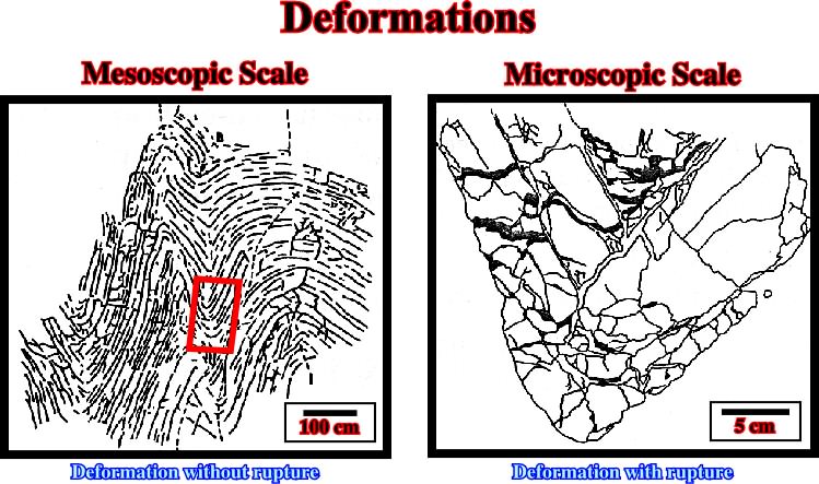
Fig. 48- At mesoscopic scale (scale of a continuous outcrop) deformation can be considered as without rupture, while a close-up of the outcrop (microscopic scale) exhibits deformation with rupture (from A. Droxler, 1982). On other hand, it is interesting to note than at mesoscopic scale, the deformation looks homogeneous, but at microscopic scale, dissolution (areas in black) clear indicates that its is not.
1.6.1- Deformations with failure
Theoretically, in homogeneous and isotropic rocks, when they fail, it is found that they break on two sets of planar shear surfaces which intersect in lines parallel to
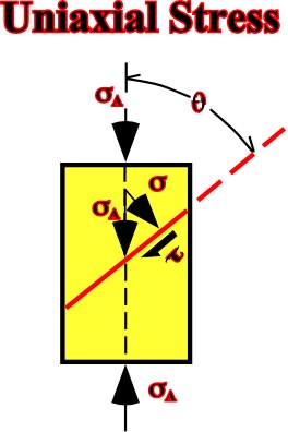
Fig. 49- An uniaxial stress
Three kinds of fractures (fig. 50) can be developed in the rocks due to mechanical failure by stress (compression):
(i) Dextral shearing fracture.
(ii) Sinistral shearing fracture.
(iii) Gash fracture (tension fracture) parallel to s1.
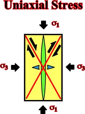
Fig. 50- Model showing the relationships between the three kinds of fractures in a rock under a uniaxial stress.
1.6.1.1- Mohr’s theory
Many theories of failure have been proposed, but the Mohr’s theory appears to be most applicable to description of the influence of pressure on failure. This theory postulates:
(i)- In a general state of stress s1 > s > s3 and,
(ii)- The intermediate stress s2 has not effect upon failure.However, it assumes that the normal stress, whether it be tension or compression, plays a role in failure as well asthe shear does.
1.6.1.2- Mohr’s circle
Mohr expressed the stress equations graphically by plotting shear stress against normal stress. Knowing the magnitude of the principal stresses, the normal and shear stresses on any plane, with values of q between 0° and 180°, can be determined using the stress equations. If the normal and shear stresses for all values of q are plotted, they form a circle, known as Mohr's circle.
The Mohr representation assumes that
(
(
(
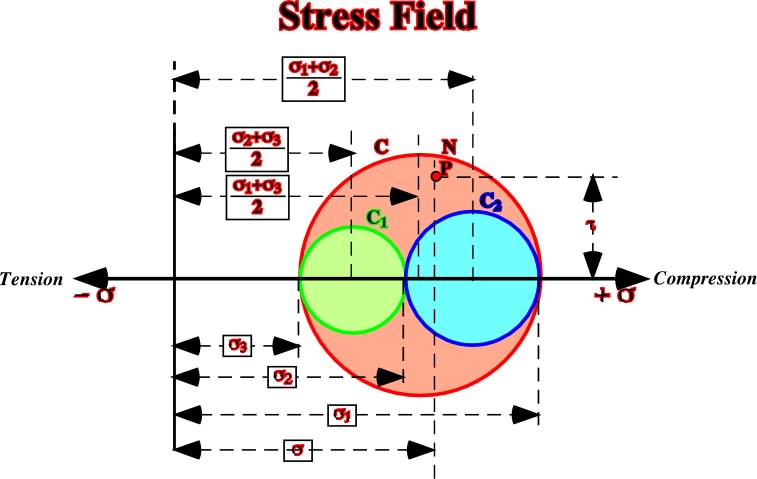
Fig. 51- Representation of the Mohr’s circle in three dimensions.
Actually, the Mohr’s circle is graphic representation of the stress field at a given point in a particular time. The coordinates of each point of the circle correspond to the stress values (tangential and normal), in a particular plane which perpendicular is at an angle f the axe
According Mohr, the graphic representation of the stresses show that the normal stress and the tangential stress in a given plane, with any orientation, can be represented by a point P within the half-moon area limited by the half-circles C1, C2 and C3.
Mohr’s theory hypothesizes that the normal stress, in compression or tension, plays a role in the failure as well as the tangential stress. Their relationships can be determined experimentally. On the other hand, the graphic representation of the stresses by circles allows determine the Mohr’s circle. As the tri-dimensional realm of the stress can be represented in a plane and the intermediated stress does not have any influence, the Mohr’s envelope can be determined by the maximum and minimum stresses.
1.6.1.3- Mohr’s envelope
Hypothesizing that all planes, under the same normal stress failure, along the same plane containing the maximum tangential stress, the intermediate stress can be neglected.
The same can be achieved by using a series of tests made under varying combinations of
t = F(
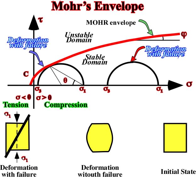
Fig. 52- The Mohr’s envelope intersects the shearing axis t at a value C called the cohesion of the material, which must be overcome priori to the development of a fracture plane.
Examples:
The Mohr’s envelop is the envelop of a series of Mohr’s circles and it corresponds to the localisation of all points which coordinates represent the failure stress, that is to say: t = F(
A) Mohr’s envelop for a marble (fig. 53).
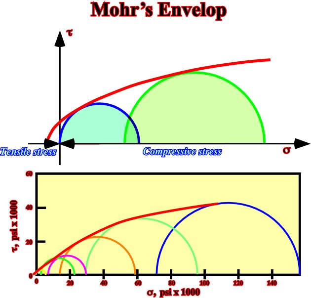
Fig. 53- Example of a Mohr’s envelop in an Hauterivian limestone. Note than failure is easier under tensile stresses than compressional stresses.
B) Mohr’s envelop for a humid claystone (fig. 54).
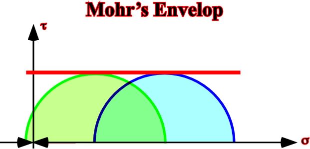
Fig. 54- Shaly sediments are so deformed than their pore-fluid cannot escape. Under these conditions, the Mohr’s envelop is a line parallel to the abscissa coordinate and its value is the tangential stress t.
C) Mohr’s envelop for a dry sandstone (fig. 55).
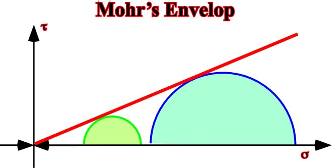
Fig. 55- As in this example the Mohr’s envelop intersects the shearing axis (ordinate) at a 0 value to t, i.e, that (
1.6.1.4- F Evolution with Increasing Stresses
The angle of failure increases with the burial of the sediments. In so far as sediments are buried,
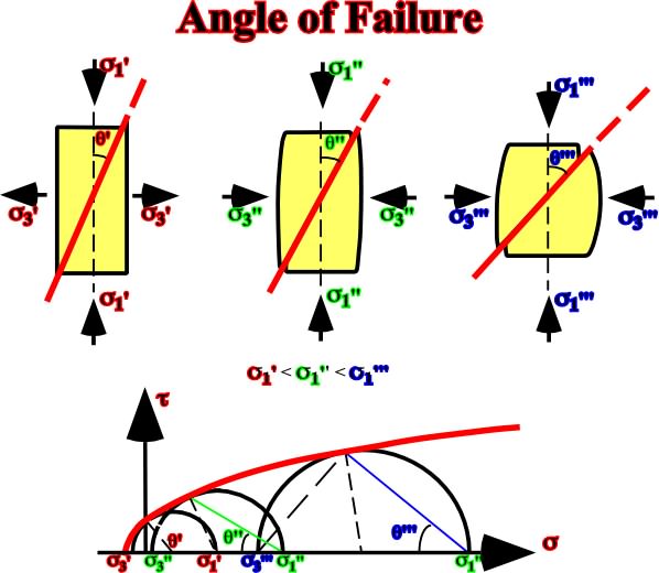
Fig. 56- The evolution of the failure angle explains why the angle of the faults planes increases in depth, that is to say, that the fault planes flattened in depth.
1.6.1.5- Pore Pressure and Rupture
The increasing of pore pressure promotes failure, as illustrated in fig. 57.
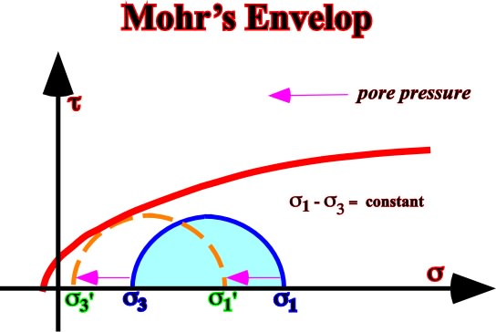
Fig. 57- Detachement planes, slopes failures and slumps, etc., can be explained by an increasing of the pore pressure.
When the confining pressure increases (
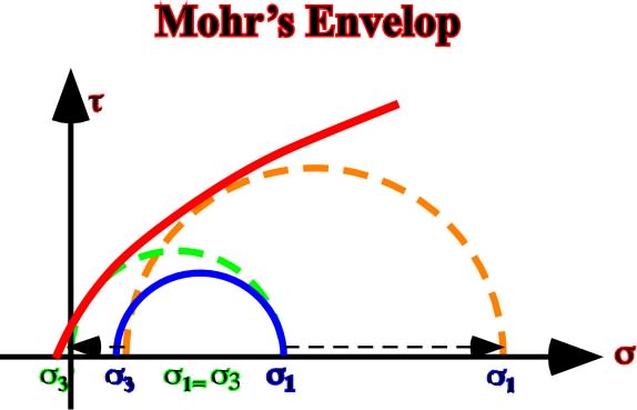
Fig. 58- This Mohr’s envelope illustrates the increasing of the confining pressure, which induces the stress-failure.
1.6.1.6- Pre-fractured Rocks
In pre-fracture rocks f1 becomes instable and the failure takes place (fig. 59).
1.6.2- Deformations without failure
As said previously, the concept of deformation without failure id depend as the scale of observation (fig. 60).
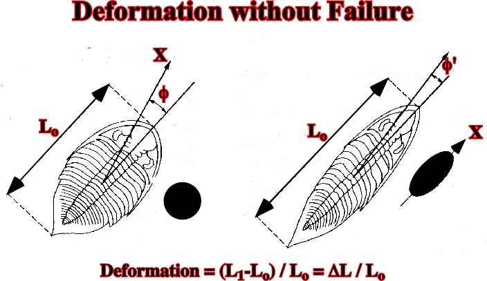
Fig. 60- Deformation without failure. The elongation can be calculate as (L1-Lo) / Lo.
For deformations without failure one can define strain ellipsoids (fig. 61) where:
-
-
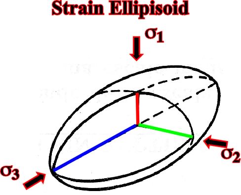
Fig. 61- In a strain ellipsoid, the direction of the maximum extension corresponds to the direction of the maximum effective stress, while the direction of the maximum shortening corresponds to the direction of the minimum effective stress, that is to say,
Deformations without failures involve:
- Inter-crystalline deformation.
- Deformation resulting from mutual grain displacement.
- Deformation resulting from pore collapse.
- Deformation resulting from dissolution and re-crystallization: the mineral solubility depends on the mechanical stress and t, P, T.
Deformations without failure occur often in limestone due to dissolution along the contact between the grains and re-crystallization. Recrystal-lization takes place within the pores (fig. 62.A). In absence of pores, recrystallization takes place along the charge contact between the grains (fig. 62.B).
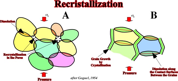
Fig. 62- Model proposed by Goguel explaining recrystallization in pore spaces.
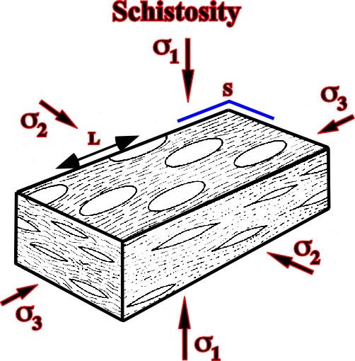
Schistosity is a good example of deformation without failure. Schistosity appears along one of the main planes of the strain ellipsoid, that perpendicular to the maximum effective stress. The direction of maximum elongation and the medium perpendicular direction are therefore on the schistosity plane (fig. 63). According to A. Heim, the longrain (side of the state = Linearstreckung), that is to say, the secondary direction of cleavage, parallel to the schistosity is more easy than transversally, must correspond to the maximal elongation direction.
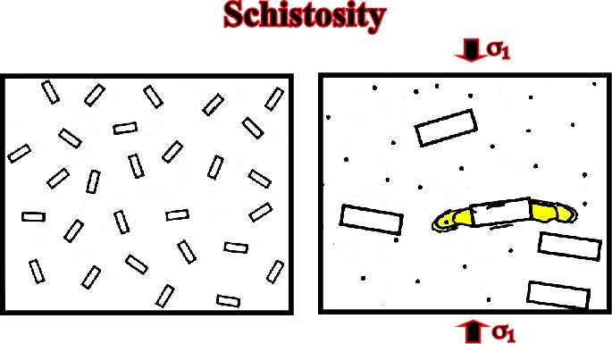
Fig. 63- The schistosity is in relation with the elongation and stretching of the rocks, that is to say, with the lengthening and mineral recrystallization along a particular direction.
Fig. 64- The schistosity plane (s3, s2) is developed perpendicular to the maximum effective stress, that is to say,
Stylotisation (fig. 65) can be considered an example of deformation without failure.
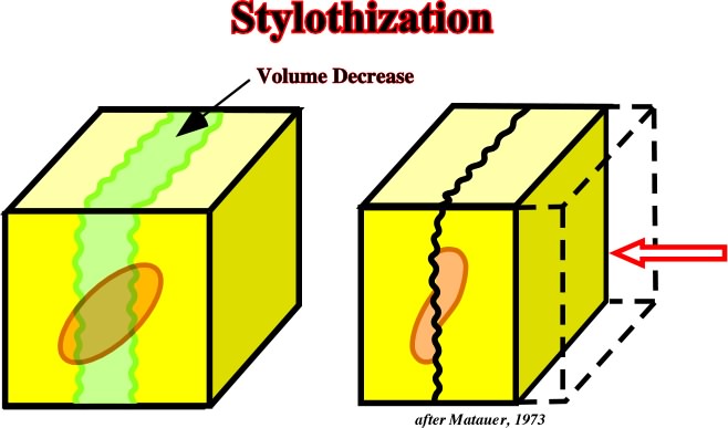
Fig. 65- Styloliths are a consequence of mineral dissolution perpendicular to the maximum effective stress.
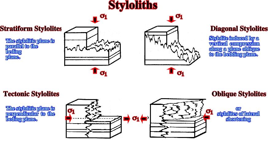
Fig. 66- Different type of styloliths associated with the maximum effective stress, ![]() 1.
1.
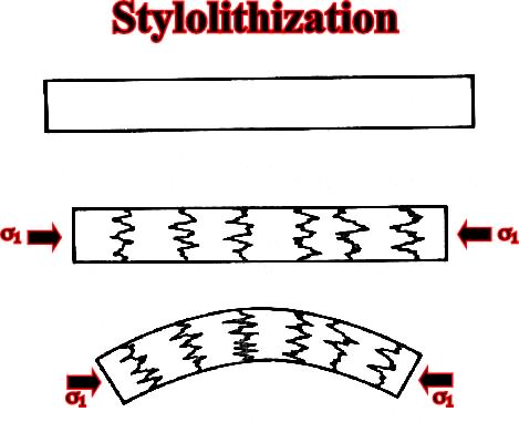
Fig. 67- Stylolithization that appears in the onset of deformation.
to continue press
next
![]()
Send E-mail to ccramez@compuserve.com or cramez@ufp.pt with questions and comments about these notes.
Copyright © 2001 CCramez
Last update: March, 2006