Diffractions occur with all waves, including sound waves, water waves, and electromagnetic waves such as visible light, x-rays and radio waves. As physical objects have wave-like properties (at the atomic level), diffraction also occurs with matter and can be studied according to the principles of quantum mechanics.
At abrupt discontinuities in interfaces or structures whose radius of curvature is shorter than the wavelength of incident waves, the law of reflection and refraction no longer apply. Such phenomena give rise to a radial scattering of incident seismic energy known as diffractions (Plate 58).
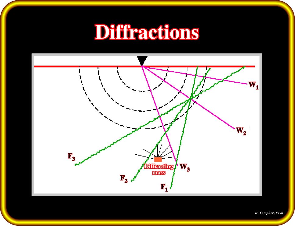
Plate 58- This plate illustrates the front of all incident waves, propagating through a homogeneous, isotropic medium obeying the principle defined by Huygens: (i) whether on a plane or an uneven disturbed surface, or as an isolated point mass, points struck by an incident wave behave as new emission sources and radiate energy in all directions on a spherical front ; (ii) for a continuous surface, most of the energy so emitted by adjacent points, actually cancels out ; (iii) the reflected ray path reaches the receiver, in most cases, as a first arrival. In classical physics, the diffraction phenomenon is described as the apparent bending of waves around small obstacles and the spreading out of waves past small openings.
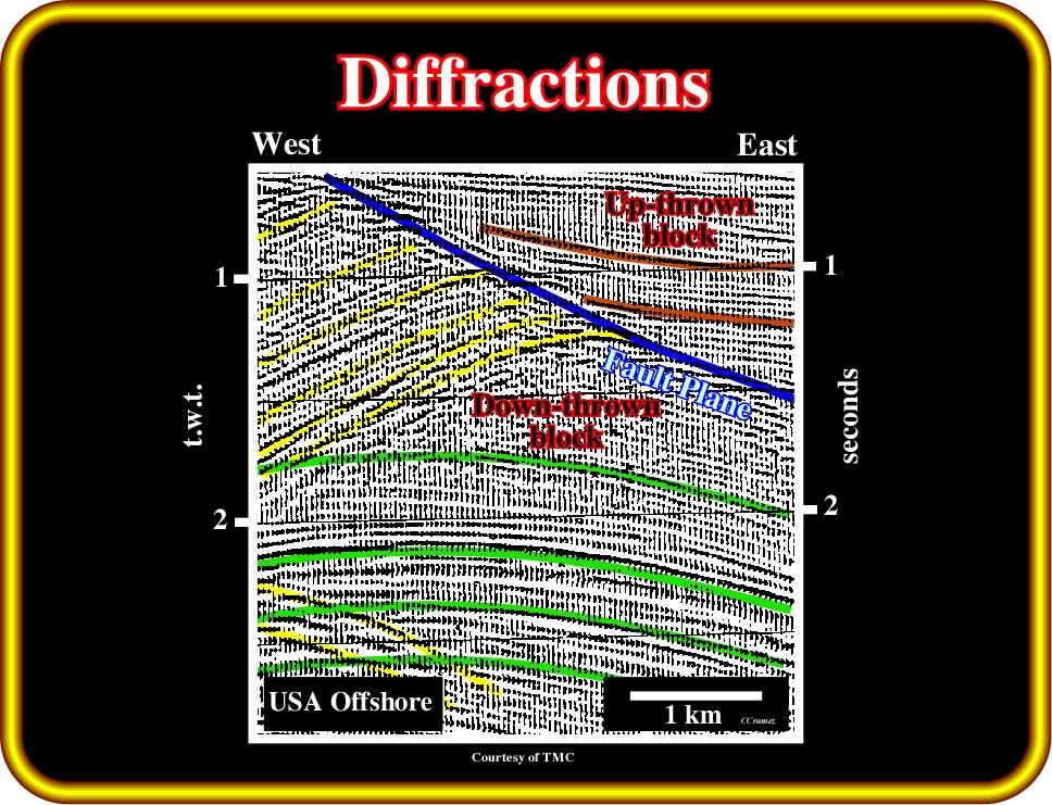
Properly speaking, diffractions are considered as noise but they could help to interpret discontinuities on unmigrated data. A hyperbolic pattern, on a nonmigrated times section, however, may be of use to the interpreter as it points out the existence of subsurface discontinuities (Plate 59).
Plate 59- This unmigrated seismic section shows a great number of diffraction patterns pointing to the existence of a discontinuity between two fault blocks. On the left block (hangingwall), it should be noticed that diffraction amplitudes are greater that reflection amplitudes. On the lower left corner, the right leg of a diffraction is probably originated from a point located off the plane of the section.
A diffraction from a given subsurface point persists when the wave length of the striking energy is greater than the longest dimension referred to underground object and cancellation from other lateral sources cannot occur. In other words, a diffraction is produced by the incidence of a wave front acoustic impedance discontinuity of limited extent at the scale of the section, which could be assimilated to a point mass.
- This could be either an isolated speck in space or the intersection of a linear event (dike, the apex of a high angle fold, a fault plane, etc.) with the plane of the section.
- Diffractions may also arise from the intersection of two apparently separated markers. This is often the case when reflection from the upthrown and the downthrown fault blocks bounces off the plane of a fault.
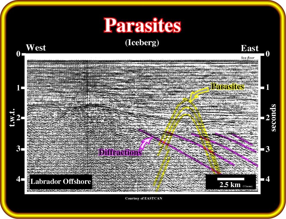
Plate 60 - On this unmigrated seismic line from Labrador Sea (Atlantic-type margin overlying rift-type basins) parasites (in yellow), induced by an iceberg, are quite evident. Ind fact, at the time of shooting, an iceberg was located no more than 1000 meters from the seismic vessel. Diffractions associated with the top of the basement (Precambrian supracrustal rocks, in this particular example) are, also, quite obvious. Notice that, on the migrated version of this line, the downward hyperbolic geometry of the parasites chances into an upward hyperbolic geometry. Parasite diffractions can be associated with: (i) airwaves, (ii) surface waves, (iii) Ambient noise (sea, wind, boats, icebergs, etc.).
Diffractions may originate in the subsurface from the edges of faulted blocks (Plate 59) or they may come from sources much closer to the surface. In marine seismic for instance, floating objects, such as ships, icebergs or wrecks on the ocean floor, often produce diffractions (Plate 60). As long as diffractions are originated from objects within the plane of the seismic section, migration (when the correct velocities are used) collapses all the energy and focuses the hyperbola on a single point at its apex. Hence, diffractions are only visible on seismic data prior to migration. Unmigrated sections may then be useful to locate local discontinuities. Common sources of diffraction in the ground include edges of faulted layers and small isolated objects, such as boulders, icebergs, etc.
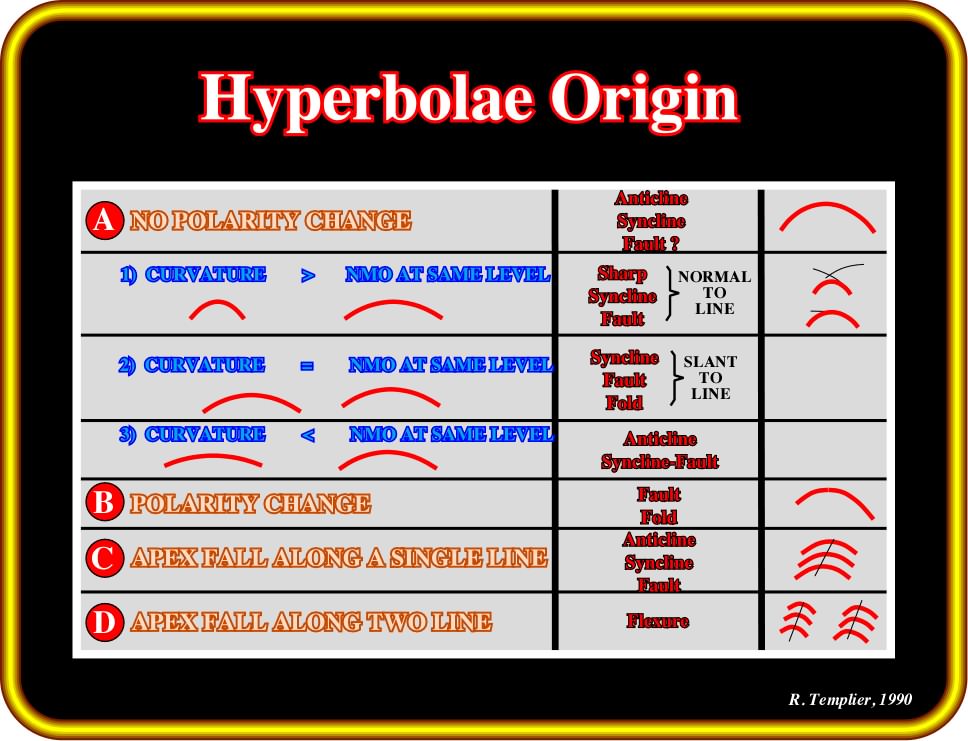
Plate 61- This table gives some of the criteria useful to interpret hyperbolic patterns on an unmigrated section. The elements considered here are the polarity (as it changes from one leg of the conic to the other) and the curvature as compared to the NMO (normal move-out) hyperbola at the same depth normal moveout correction (NMO) is a stretching of the time axis to make all seismograms look like zero-offset seismograms. This kind of correction may be done to common-shot field profiles or to CMP gathers (a common-midpoint gather holding data with only one velocity should stack OK without need for antialiasing. It is nice when antialiasing is not required because then high temporal frequencies need not be filtered away simply to avoid aliased spatial frequencies. When several velocities are simultaneously present on a CDP gather, we will find crossing waves. These waves will be curved, but aliasing concepts drawn from plane waves are still applicable, http://sepwww.stanford.edu/public/docs/sep73/jon3.trimo/paper_html/node8.html. NMO applied to a field profile makes it resemble a small portion of a zero-offset section (distance between source and receiver is zero).
On Plate 61, are summarized the more frequent origins of hyperbolae that one can find on unmigrated seismic lines. Generally, hyperbolas can be created by:
(i) Folds (when the axial plane is vertical, the hyperbola do not show polarity change; the curvature must be compared to the NMO hyperbolae at the same depth) ;
(ii) Faults and Flexures.
It must be noticed that the criteria illustrated on the previous plate are not sufficiently discriminatory. Simpler criteria do exist to distinguish a syncline from an anticline and a fault from a fold, as illustrated in Plate 62.
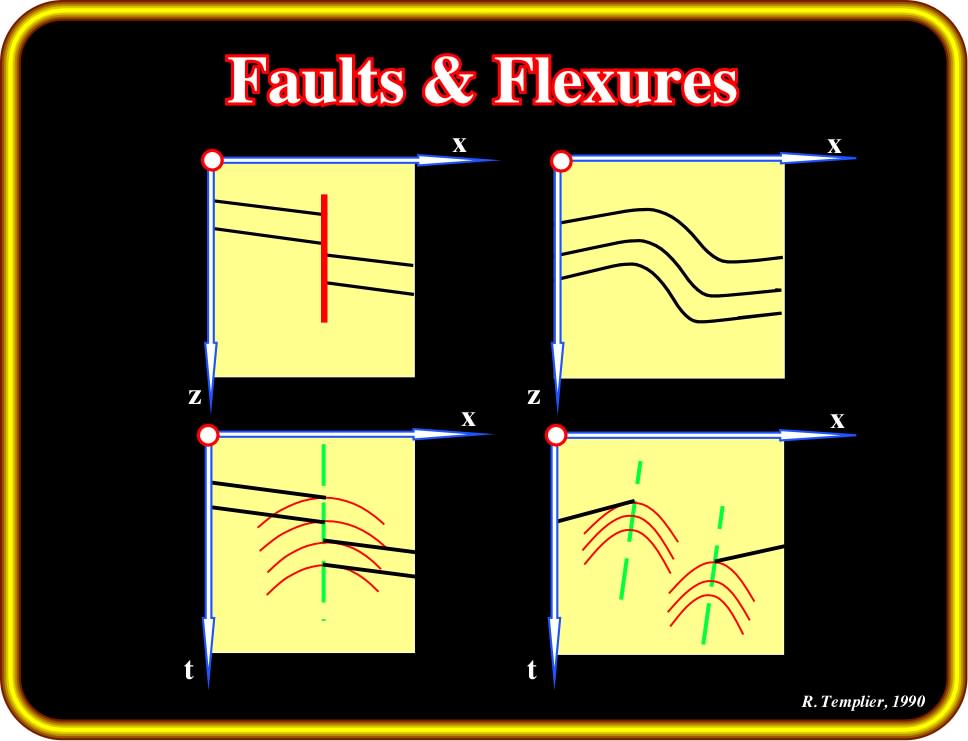
Plate 62- The presence of superposed hyperbolas on a seismic line may assist in correctly interpreting a fault or a flexure. In the case of a fault (on the left), hyperbolae line up vertically over the intersection of the fault plane with the plane of the section. In the case of a flexure, two sets of displaced hyperbolas pinpoint the top and the base on the flexure. Interpreters should not forget that vertical normal faults do not exist in Geology. In fact, the aim of a normal fault is to lengthen the sediments. A vertical normal fault does not lengthen or shorten the sediments so it is a nonsense. In addition, it requires space in depth, and as my old professor of geology said, the hell is full so there is not space for vertical normal fault. Only very locally, the geometry of a normal fault plane is vertical. By definition, the dip of a normal fault must increase with depth, that is to say, the hade of the fault plane (angle with the vertical measured perpendicular to strike) must increase, in order to length the sediments. On the other hand, as the compressional wave velocity of the sediments increase with depth, and seismic lines are time-profiles, in a seismic line all fault planes must flatten in depth.
In order to examine the seismic image of a fault, we will consider the geological model illustrated on Plate 63, where:
(i) The fault plane is vertical (local geological situation, since a macroscopic scale all normal fault planes are curve in depth, in other words, a vertical normal fault is a physical impossibility vue that is this case there is no lengthening) ;
(ii) The upthrown and downthrown fault blocks have the same dip ;
(iii) A seismic profile (line C) intercepts the fault plane with an angle
.
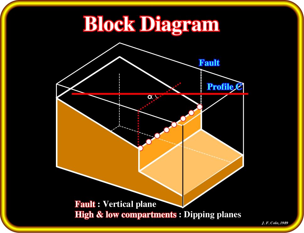
Plate 63- This block diagram illustrates the geological model used to study the seismic image of a normal fault. In spite of the impossibility to develop large-scale vertical normal fault planes, for simplicity, we assume a local vertical fault plane geometry (this geometry corresponds to a strike slip fault. In this model the fault blocks have the same dip. On should not forget that normal faults develop to lengthened the sediments. A fault with a vertical fault plane (at macroscopic scale) do not lengthen and do not shorten, so likely it corresponds to a pure strike slip fault (very rare on the field).
The time response of such a model is depicted on Plate 64:
A) On the upper part of the Plate 64:
- “BC” is the trace of the seismic line on the ground surface ;
- “F” is the trace of the vertical fault plane on the ground surface ;
- “
” is the intersection angle between the fault plane and the seismic line.
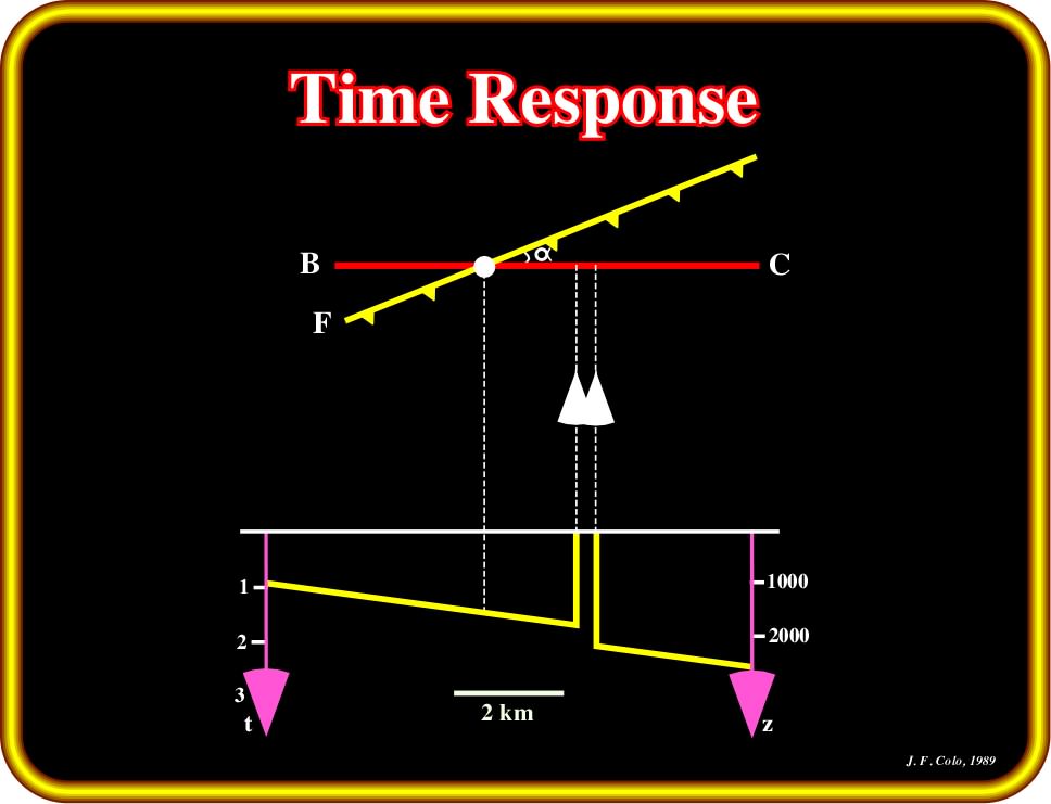
Plate 64- The time answer of the previous faulting geological model is depicted on the lower part of this sketch. On top, the traces of the seismic line and the vertical fault plane are represented. The location of the fault is displaced down-dip. In addition, it corresponds to a blind zone rather than a vertical reflection.
B) On the lower part, is depicted the time response (seismic line):
- The fault plane is not located right under the corresponding shot point on the surface ;
- The fault plane is slightly displayed to the right (down-dip) ;
- The fault is not imaged as a vertical reflection segment;
- A blind zone separates the two fault-blocks.
Similarly to what we have already seen, in the case of migration with dipping beds, the shortest travel times (traveling paths perpendicular to the marker) are situated on the vertical plane of the section, but to points up-dip of it. A depth-section response on a vertical plane is shown on Plate 65.
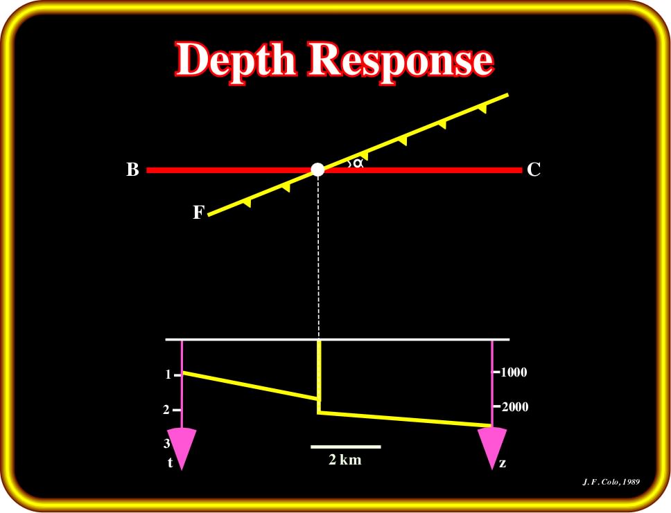
Plate 65- The lower part of this sketch shows the theoretical vertical depth-section corresponding to the recorded section of the previous theoretical model. The upper part shows a plane view of the position of the actual reflection points of the marker as projected on the ground surface.
Let's see a seismic example in which such a geological model can be used (Plate 66).
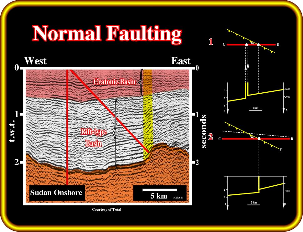
Plate 66- On this line from onshore Sudan, that is to say, a seismic line shot in a rift-type basin (Bally’s basin classification) overlain by a quite thin cratonic basin (sag phase), a blind zone (yellow) is developed between the up-thrown and down-thrown blocks of the normal fault. One can conclude that: (i) the seismic profile intersects the fault plane at certain angle, (ii) the true position of the fault, with respect to the profile, is to be found rightward of its apparent position on the time section.
The tentative interpretation of this seismic line is justified by:
The disturbed zone to the right could either be a vertical fault or a flexure.
In fact, as illustrated below (Plate 67), several vertically aligned hyperbolae are visible:
(i) Their curvature conform with the curvature of dynamic corrections (in overlay) ;
(ii) Likely that they are in fact diffraction images ;
(iii) As only one set of superimposed hyperbolas is present (and not two), the pattern most probably indicates the presence of a fault and not a flexure on the seismic line ;
(iv) The apparent velocity, as measured on the hyperbolic pattern, is higher than the NMO velocity at the corresponding depth. This would indicate the line is not perpendicular to the fault plane.
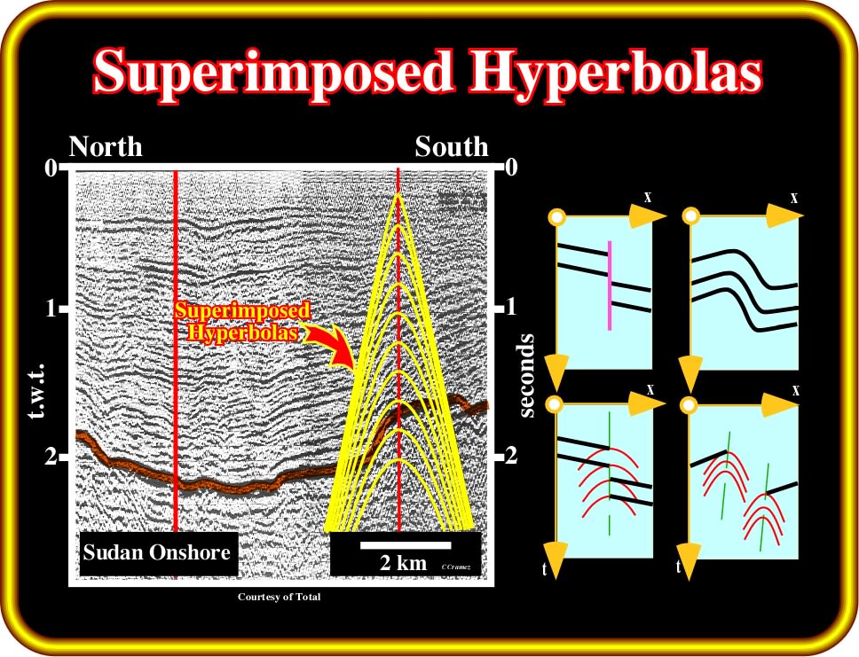
Plate 67- As just one set of superimposed hyperbolas fits the diffraction recognized on the seismic line, the most likely meaning of such diffractions is the presence of a fault plane (the geometry of this fault plane is quite local; normal fault planes are vertical, just locally, since the dip flattens in depth).
Before studying the next geological normal faulting model, it will be interesting to analyze the interpretation consequences of the obliquity of seismic profiles in vertical (local) normal fault planes (Plate 68).
Plate 68- This sketch tackles a common problem in seismic interpretation. The plane view shows, in red, the projection on the ground surface of a fault plane “F”, and in blue, is indicated the location of three distinct seismic profiles. One is oblique to the fault, the others are perpendicular to it in the direction of the dip.
The black lines indicate the possible interpretations of the fault on the basis of the recorded data :
- Lines B and C correctly place the fault at its true position ;
- For the reasons we have examined, A displaces the fault updip along the line of a distance that depends on the angle of inclination of the reflecting bed ;
- If a second fault exists in the area, and is recorded further down on C, the interpreter would naturally tend to draw a straight line joining the fault indications as recorded on the three profiles.
- The correct correlation however is the curved line shown in the plate.
If the bed is dipping, all three lines will displace the fault. Lines B and C will migrate the fault to its true position, but A will not because the reflecting points are off the plane of the section.
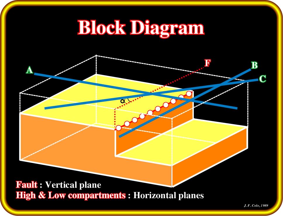
Plate 69- This block diagram illustrates a geological model, in which a local vertical normal fault displaces horizontal faulted blocks. The block diagram is crossed by three seismic lines. One of the lines is perpendicular to the fault plane (line A). The line B is parallel to the fault plane and the line C is oblique.
The above geological normal faulted model (Plate 69) of a normal faulting can be characterized by:
(i) A vertical fault plane, which is a local geological situation ;
(ii) Horizontal bedding planes ;
(iii) Three seismic profiles ;
(iv) One of the seismic profiles is parallel to the strike of the fault ;
(v) The others profiles are perpendicular and oblique to the fault.
The time and depth-seismic responses of this simple geological model are pictured on Plate70.
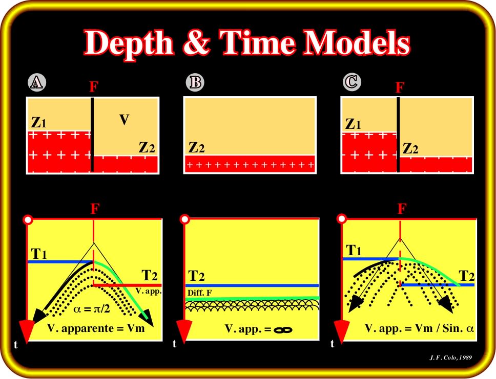
Plate 70- In these sketches are illustrated the depth (local models) and time responses along the seismic profiles A (perpendicular to the fault plane), B (parallel to the fault plane crossing just the downthrown block, since the fault plane is vertical), C (oblique to the faulte plan crossing both faulted blocks) the geological model proposed on Plate 69.
Profile ”A” (perpendicular to the fault plane):
- The position of the fault is the same on the depth and on time sections ;
- The apparent velocity corresponding to the hyperbolic diffraction patterns is the same as the average velocity through the formation ;
Profile “B” (parallel to the fault):
- The reflections from the surface of the down-thrown block and from the edge of the up-thrown block are both horizontal and visible ;
- The reflections are accompanied by a diffraction pattern whose envelope is displaced relative to the edge of the fault ;
Profile “C” (oblique to the fault plane):
- Since the assumed model has 0 dip, the time image of this plane corresponds to its true depth position even though the seismic profile is slanted with respect to the fault plane ;
- The apparent velocities, however, as determined by the diffraction hyperbolae, deformed by the skew of the line, are then the average velocity within the formation ;
In order to avoid misleading interpretations in which diffractions are taken as geological events, the diffraction characteristics generated at the end of a layer and at the end of a faulted layer we summarized on Plates 71-72;
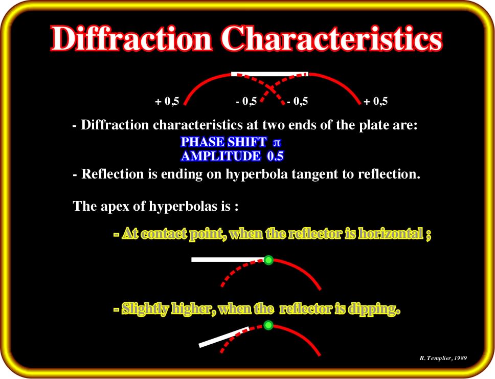
Plate 71- This sketch illustrates the main characteristics of diffractions associated at the terminations of a sedimentary layer. In other words, reflection terminations are underlined by diffractions (hyperbolas) with opposite polarities and a phase shift. The hyperbolas are tangent to reflections with the apex at the contact point when the reflection is horizontal and slightly higher when the reflector is tilted.
Diffraction characteristics:
- The polarity of the hyperbola legs, outward from the slab, has the same polarity as the reflection from the slab ;
- The polarity of the hyperbola legs, beneath the slab, is opposite to the polarity of the reflection from the slab ;
- The amplitude of the diffraction hyperbola is half the absolute value of the amplitude of the reflection from the truncated layer ;
- A horizontal reflecting truncated layer is tangent to the diffraction hyperbola at its apex ;
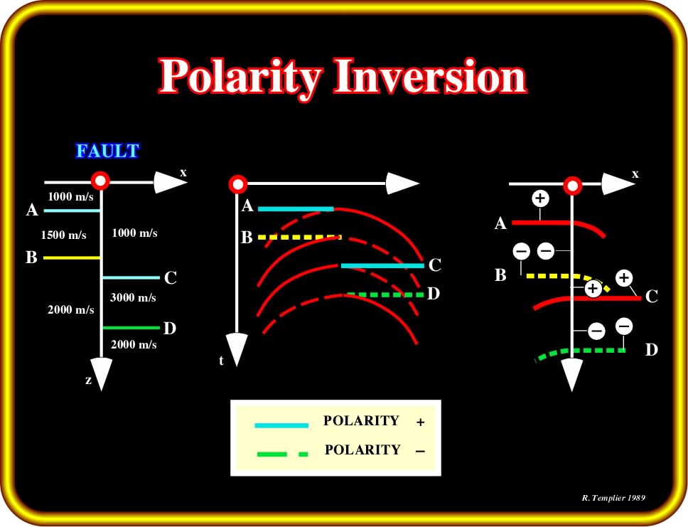
Plate 72- Diffraction characteristics in the case of a faulted layer. On the upthrown faulted block, the interfaces A and B create a seismic marker ending by a diffraction branch looking to the downthrown block. On the contrary, on the downthrown faulted block, the seismic markers associated the interfaces C and D terminate (against the fault block) by diffraction branches looking toward the fault plane. Notice that this geological model is valid just at mesoscopic scale (local model) since at macroscopic scale all normal faults planes dip to the dowthrown faulte blocks flattening in depth.
- A dipping reflecting truncated layer intercepts the hyperbola down from the apex of the conic.
- A reflecting truncated layer, with positive acoustic impedance contrast, at its top, and a negative at its base, has been faulted and the two blocks have been displaced.
- Each severed edge of the marker acts as a separate layer and generates, outwardly, an hyperbola leg of the same polarity as the slab and, beneath it, one of opposite polarity to the marker.
to continue press
![]()