According to Nettleton (1976), any conceivable property or process, which can be measured or carried out at above the surface, and, which is affected by the nature of rocks through a cover of hundreds to many thousands of feet of intervening rocks, may be made the basis of a method of geophysical prospecting. Fundamentally, there are two main families of geophysical surveying (P. Kearey and M. Brooks, 1993):
(i) Natural Field Methods
They utilize the gravitational, magnetic, electrical and electromagnetic fields of the Earth. They look for local perturbation in these naturally occurring fields that may be caused by concealed geological features.
(ii) Artificial Field Methods
They involved the generation of local electrical or electromagnetic fields that may be used analogously to natural fields. In the most important group of geophysical methods, the generation of seismic waves and their propagation velocities and transmission paths through the subsurface, are mapped to provide information on the distribution of the geological boundaries at depth.
A wide range of physical surveying methods exists. For each method there is an operative physical property to which the results are sensitive:
a) Seismic Method
It measures the travel times of reflected or refracted seismic waves using as operative properties the density and elastic moduli, which determine the propagation velocity of seismic waves.
b) Gravity Method
It measures the spatial variations in the strength of the gravitation field of the Earth. The operative physical property is the density.
c) Magnetic Method
It measures the spatial variations in the strength of the magnetic field. The operative physical property is the magnetic susceptibility and remanence.
d) Radar Method
It measures the travel times of reflected radar pulses. The operative physical property is the dielectric constant.
In the majority of geophysical survey methods, explorationists are mainly interested in geophysical anomalies, i.e., local variations in the measured parameter, relative to some normal background value. Such variations are attributable to a localized subsurface zone of distinctive physical properties and possible geological importance. However, geophysical interpretation is quite ambiguous. In fact, here are two kind of problems in geophysical surveying:
-If the internal structure and physical properties of the Earth were precisely known, the magnitude of any particular geophysical measurement taken at the Earth‘s surface could be predicted uniquely. Thus, for example, it would be possible to predict the travel time of a seismic wave reflected off any buried layer or to determine the value of the gravity or magnetic field at any surface location ( P. Kearey and M. Brooks, 1993).
- However, often, in geophysical surveying, the problem is the converse of the above, namely, to deduce some aspects of the Earth’s internal structure on the basis of geophysical measurements taken at (or near to) the Earth’s surface.
The former type of problem is known as a direct problem, the latter as an inverse problem. Whereas direct problems are theoretically capable of unambiguous solutions, inverse problems suffer from an inherent ambiguity, or non-uniqueness, of conclusions that can be drawn. Let’s see the examples proposed by P. Kearey and M. Brooks (1993):
a) Direct Problem
The travel time of an echo-sounding is measured and converted into a water depth, multiplying the travel time by the velocity with which sound waves travel through water, i.e. 1500 m/s. Thus an echo time of 0.10s indicates a path length of 0.10 x 1500 = 150 m, or a water depth of 150/2 = 75 m, since the pulse travels down to the sea bed and back up to the transducer located in the ship.
b) Inverse Problem
Using the same principle, a simple seismic survey may be used to determine the depth of a buried geological interface (e.g. the top of a limestone layer). This would involve generating a seismic pulse at the Earth’s surface and measuring the travel time of a pulse reflected back to the surface from the top of the limestone. However, the conversion of this travel time into a depth requires knowledge of the velocity with which the pulse travel along the reflection path and, unlike the velocity of sound in water, this information is generally not known. If a velocity is assumed, a depth estimate can be derived but it represents only one of many possible solutions.
Although the degree of uncertainty in geophysical interpretation can often be reduced to an acceptable level by taking additional field measurements, the problem of inherent ambiguity cannot be overcome. The general problem is that significant differences from an actual subsurface geological situation may give rise to insignificant, or immeasurably small, differences in the quantities actually measured during a geophysical survey. Since a unique solution cannot, in general, be recovered from a set of field measurements, geophysical interpretation is concerned either to determine properties of the subsurface that all possible solutions share, or to introduce assumptions to restrict the number of admissible solutions (Parker, R. L., 1977).
Practically, all geophysical search for hydrocarbons depends on a very few basic physical principles:
(i) Elastic waves,
(ii) Magnetics,
(iii) Gravity,
which characterize the three main prospecting methods:
-Seismic methods -Magnetic methods -Gravimetric methods.
Seismic methods are concerned with the measurement and analysis of waveforms that express the variation of some measurable quantity as a function of distance and time. The quantity of information, and in some cases, the complexity of data processing to which these waveforms are subjected is such that the processing can only be accomplished effectively and economically by digital computers. The two basic parameters of a digitizing system are:
1) Sample Precision or Dynamic Rang
The dynamic range, which is expressed in decibel (dB), is the expression of the ratio of the largest measurable amplitude to the smallest measurable amplitude in a sample function.
2) Sampling Frequency
The sampling frequency is the number of sampling points in unit time or unit distance. Ex: if a waveform is sampled every two milliseconds (sampling interval), the sampling frequency is 500 samples per second or 500 Hz.
If the frequencies above the Nyquist frequency* (the frequency of half the sampling frequency; Nyquist interval is the frequency range from zero to the Nyquist frequency) are present in the sampled function, a serious form of distortion known as aliasing occurs. To overcome this problem, either the sampling frequency must be at least twice as high as the highest frequency component present in the sampled function, or the function must be passed through an anti-alias filter prior to digitalization.
*Nyquist frequency is the frequency of half the sampling frequency. Nyquist interval is the frequency range from zero to the Nyquist frequency.
Gravimetry and Magnetics are potential field methods. They have their fundamentals in the mathematical theory of potential fields. So, gravitational or magnetic forces are, in a given direction, the derivative, or rate of change, in that direction, of the gravitational or the magnetic potential.
In these notes, we concentrate mainly in the seismic method, and particularly seismic reflection and geological interpretation. Magnetic and gravitational, i.e., the potential methods will be just briefly outlined.
Gravimetry and Magnetics, i.e., the potential methods, are based on the potential theory. They have certain elements in common. Nevertheless their applications in oil exploration are quite different:
(i) Measured gravity effects are caused by sources that may vary in depth from the grass roots down.
(ii) Sedimentary rocks, which are the ones in which generally hydrocarbon may occur, nearly always are less magnetic than the underlying basement (usually igneous or metamorphic rocks).
(iii) Magnetic effects are not too influenced by the sediments. One can say that its effects are almost the same as if the sediments were not present.
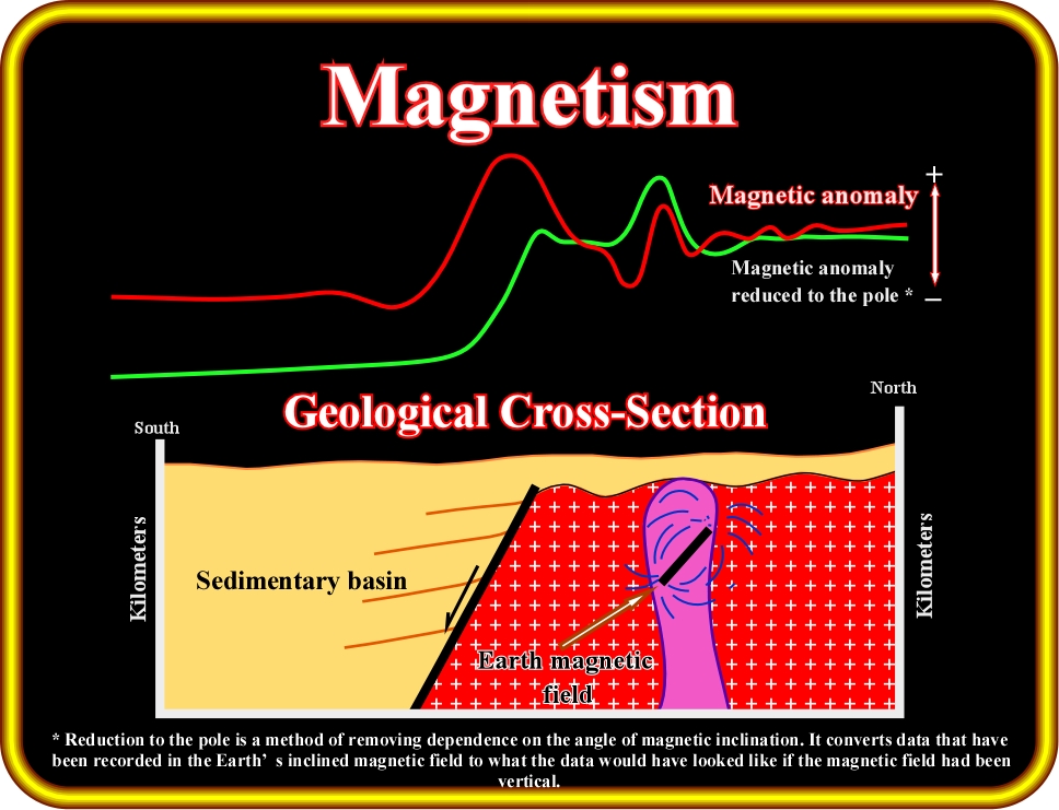
Plate 25 - This figure depicts the main principles of the magnetic method. A survey is made with a magnetometer on the ground or in the air. The survey yields local variations, or anomalies, in magnetic-field intensity. Then, the anomalies will be compared and interpreted, in relation to a geological model, as to the depth, size, shape, and magnetization of geologic features causing them.
Petroleum geologists and geophysicists, often called Explorationists, should not forget that these methods are deterministic. Such a feature implies an important epistemological limitation:
Gravimetric or magnetic maps can just falsify or corroborate geological models (indirect interpretation). They cannot or should not be used to make geological interpretations.
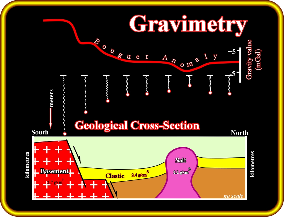
Plate 26- The relatively low density of salt with respect to its surroundings renders the salt dome a zone of anomalously low mass. Earth‘s gravitational field is perturbed by subsurface mass distributions and the salt dome therefore gives rise to a gravity anomaly that is negative with respect to surrounding areas, as illustrated on the Bouguer anomaly. As gravimetry is a deterministic method, that is to say, an a priori geological interpretation is required, which, then, can be refuted or corroborated by the gravimetric data.
Gravity and magnetic processing sequences can be summarized as follows:
a) Pre-Processing
(i) Reading/Converting Field Tapes, (ii) -Line Definition, (iii) Data Editing, (iv) Digitizing (if unrecordable or not recorded digitally), (v)- Positions, Shot-points, and Time (if acquired on a seismic operation).
b) Basic Processing
- Meter Calibration, Base Constants and Drift.
Correction for instrumental drift is based on repeated readings at a base station at recorded times throughout the day.
- Base Station Magnetic Observation and Diurnal.
The effects of diurnal variation may be removed in several ways. For magnetics (land) a method similar to gravimeter drift monitoring may be employed in which the magnetometer is read at a fixed base station periodically throughout the day.
Magnetometers do not drift and base readings are taken solely to correct for temporal variation in the measured field. Magnetic effects of external origin cause the geomagnetic field to vary on a daily basis to produce diurnal variations. Under normal conditions (quiet days), the diurnal variation is smooth and regular and has small amplitude, being at maximum in Polar Regions. Disturbing days are distinguished by far less regular diurnal variations and involve large, short-term disturbances in the geomagnetic field, with big amplitudes (magnetic storms).
- Intersection Determination.
- Misty Adjustments.
- Systematic Corrections
- Random Error Correction
- Profiling.
- Gridding and Contouring.
- General Reduction
Before the results of gravity or magnetic surveys can be interpreted, it is necessary to correct them for all variations in the Earth‘s potential fields:
- International Gravity Formula
It is a formula expressing theoretical gravity on the surface of a specified reference ellipsoid as a function of latitude.
- Earth’s Normal Magnetic Field
The International Geomagnetic Reference Field (IGRF) defines the theoretical dipolar undisturbed magnetic field related to neck at any point on the Earth's surface. In magnetic surveying, the IGRF is used to remove from magnetic data those magnetic variations attributable to this theoretical field.
- Correction Sun / Moon motion
- Eotovos Correction
In gravity measurement, on a moving platform (ship or aircraft) a correction, for centripetal acceleration caused by east-west velocity over the surface of the rotating Earth, is necessary.
- Free Air Correction
This correction corresponds to the natural decreasing of the field with elevation, i.e., the distance between observation point and the geoid.
- Bouguer and Terrain Corrections
The Bouguer correction is a correction made to gravity data for the attraction of the rock between the station and the datum elevation (commonly sea level). If the station is below the datum elevation, for the rock missing between the station and the datum, the Bouguer correction is 0.01276 ph mgal/ft, or 0.04185 ph mgal/m, where p is the specific density of the intervening rock and h is the difference in elevation between station and datum.
Terrain corrections should be applied if the actual topographic or bathymetric surface deviates significantly from the infinite Bouguer slab. For land and underwater stations, this correction is positive because both high areas above the station and low areas below it causes a lower gravity reading than would have been observed if the land were flat. For the sea stations over relatively deep water, a negative correction may be required because of the positive influence surrounding rocks above the station water depth.
Terrain correction can be made either manually or by computer by dividing the topography into compartments and summing the individual effects at each station. This requirement can add significantly to the cost of processing gravity data.
This method is based on measurements of small variations in the magnetic field:
- Indeed, as most sedimentary rocks are nearly non-magnetic, all inhomogeneous composition of basement rocks, or important topographic relief of the basement surface cause variations in the magnetic field.
- These variations can be measured by sensitive magnetometers at surface or, more commonly, by suitable instruments carried in an aircraft or behind a ship.
The measured variations in the magnetic field are interpreted in terms of the probable distribution of magnetic material below the surface, which in turn is the basis for inferences about the probable geological conditions (Plate 7).
Negative anomalies occur on the north sides of the buried magnetic masses in the northern hemisphere, and on the south side in the southern hemisphere. Maximum anomaly occurs at the poles and minimum anomaly at the equator.
The most important results of magnetic interpretation are:
(i) Depth determination of the basement rocks, or the thickness of sediments, and
(ii) Determination of local paleo-highs of the basement surface.
The interpretation of magnetic anomalies is similar, in its procedures and limitations, to gravity interpretation as both techniques utilize natural potential fields based on inverse square laws of attraction. The force F between two magnetic poles strengths m1 and m2 separated by a distance r is given by:
F =
m1m2 /4
r2
where,
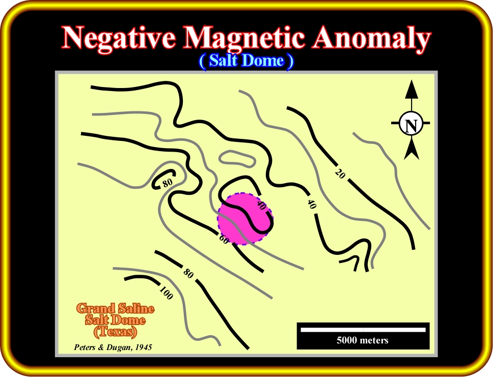
Plate 26.1- The negative magnetic susceptibility of salt causes a local decrease in the strength of the Earth‘s magnetic field in the vicinity of a salt dome. Readings have been corrected for large-scale variations of the magnetic field with latitude, longitude and time. The contours reflect only those variations resulting from variations in the magnetic properties of the subsurface. On this map, as expected, the salt dome (in purple) creates a negative anomaly, although the magnetic low is displaced slightly from the centre of the dome.
There are several particularities, which increase the complexity of magnetic interpretation:
a) The gravity anomaly of a causative body is entirely positive or negative, depending on whether the body is more or less dense than its surroundings.
b) The magnetic anomaly of a finite body invariably contains positive and negative elements arising from the dipolar nature of magnetism.
c) The intensity of magnetization is vectorial, while the density is scalar.
d) The direction of magnetization in a body closely controls the shape of its magnetic anomaly.
For the above reasons, magnetic anomalies are often much less closely related to the shape of the causative body than are gravity anomalies. In other words:
“Bodies of identical shape can give rise to very different magnetic anomalies”
As in other potential methods, the interpretation can be:
(i) Direct or
(ii) Inverse (Indirect)
Limiting depth is the most important parameter derived by direct interpretation. It may be deduced from magnetic anomalies by making use of their property of decaying rapidly with the distance. The inverse or indirect interpretations of magnetic anomalies are made to match the observed anomaly with that calculated for a model by iterative adjustments to the model.
The sequence of a magnetic interpretation can be summarized as follows:
a) Magnetic Anomaly
About 90% of the Earth‘s field can be represented by the field of a theoretical magnetic dipole at the centre of the Earth inclined at about 11°5 to the axis the rotation.
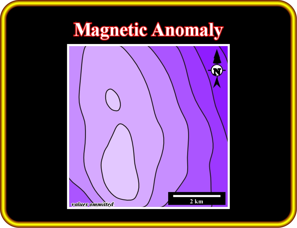
Plate 26.2- This map illustrates a magnetic anomaly. It represents the intensity of the Earth’s Magnetic field corrected for regional field (dipole effect) and diurnal (HF variations) effects. Magnetic anomalies are the difference between observed and corresponding computed values or the difference from the general surrounding values. Such differences are often induced by geological features.
- The magnetic moment of this fictitious geocentric dipole can be calculated from the observed.
- If this dipole is subtracted from the observed magnetic field, the residual field can be approximated by the effects of a second smaller dipole.
- The process can be continued by fitting dipoles of ever decreasing moment until the observed geomagnetic field is simulated to any required degree of accuracy.
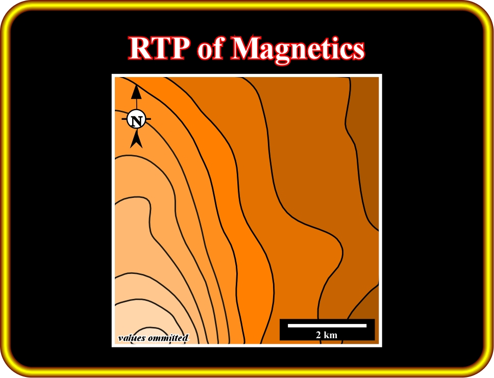
b) Reduction to the Pole (RTP) of Magnetics
Reduction to the pole involves the conversion of anomalies into their equivalent form at the north magnetic pole. This process usually simplifies the magnetic anomalies, as the ambient field is then vertical and bodies with magnetizations which are solely induced. The existence of remnant magnetization, however, commonly prevents reduction to the pole from producing the desired simplification in the resultant pattern of magnetic anomalies.
Plate 26.3- A reduction to the pole (RTP) map of magnetics, as the one illustrated above, corresponds to the conversion of the anomalies into their equivalent form at the north magnetic pole. This process usually simplifies the magnetic anomalies (Plate 26.2).
c) Reduction to the Equator (RTE) of Magnetics
In the northern hemisphere, the magnetic field generally dips downward the north and becomes vertical at the north magnetic pole. In the south hemisphere the dip is generally upward toward the north. The line of zero inclination approximates the geographic equator, and is know as the magnetic equator.
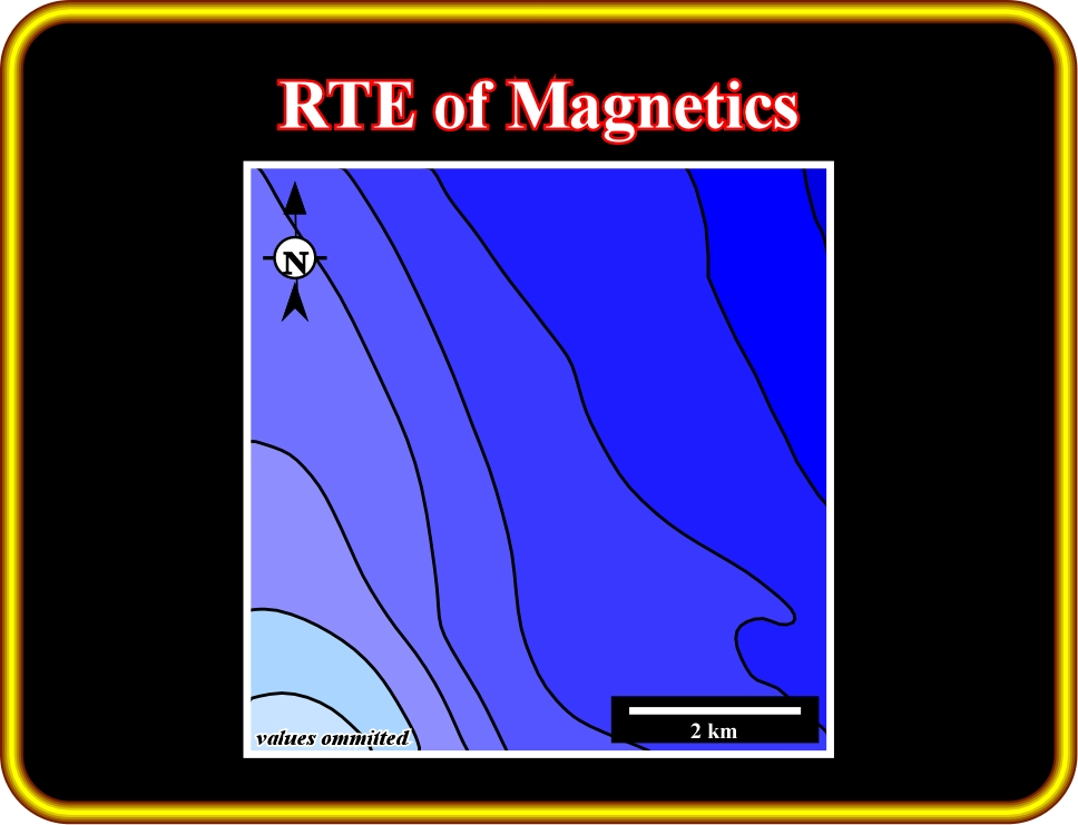
Plate 26.4- This RTE map of magnetics represents what the data would have looked like if the magnetic field had been horizontal (zero inclination). Comparing this map with the magnetic anomaly map (Plate 8), the advantages of a RTE map is quite evident.
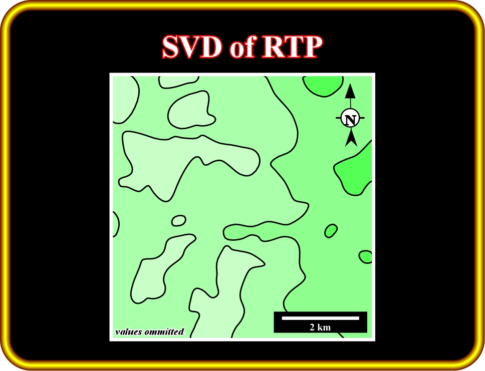
d) Second Vertical Derivative (SVD) of RTP
In geophysics, derivative maps are maps of one of the derivatives of a potential field, such as the Earth’s gravity or magnetics. The more frequent derivative maps are those of the second vertical derivative (second-derivative map), which strongly enhance the morphology of the maps and so a more accurate location of the anomalies.
Plate 26.5- the second vertical derivative (SVD) of the reduction to the pole (RTP) map enhances subtle magnetic anomalies, which can later be corroborated or not by geological data. Enhancement of classic potential fields allows a better localization of the sources. Do not forget that the derivative of a curve is its tangent. During the night, when you drive your car in a mountainous road, the light of the headlights gives the first derivative of the road, that is to say, its inclination.
The derivative of a function, as the reduction to the pole, expresses the rate of change of that function. Indeed, on the graph of the curve y = f(x), the derivative at a given point x is equal to the slope of the tangent line at the point [x, f(x)].
Admittedly, as illustrated on Plate 26.5, a derivative map enhances the anomalies, which allows a finer location of the magnetic bodies.
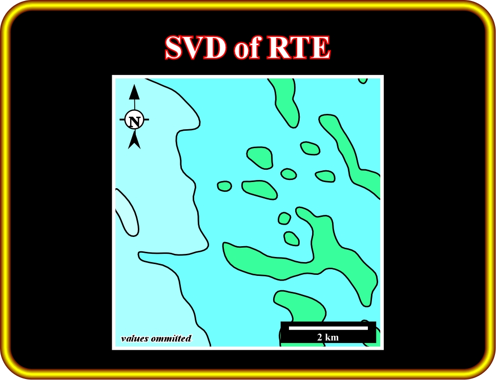
e) Second Vertical Derivative (SVD) of RTE
Second vertical derivative of the reduction to the equator maps, as that illustrated on Plate 26.6 are often made to facilitate the recognition of subtle magnetic anomalies.
Plate 26.6- This map represents the second vertical derivative (SVD) of the reduction to the equator (RTE) of the magnetic anomaly (see Plate 26.2), which enhancing the potential field switch order a better localization of the magnetic source. To understand such enhancements suppose a long quite flat road, in which several bumpers were put in place by the local police. When driving during the daytime, the bumpers, when not painted, are difficult to locate. However, when driving during the night, they are easily located by the abrupt changes of the lights of headlights of the car moving in opposite direction (first derivative of the road).
f) Magnetic Interpretation
In magnetic interpretations, the problem of ambiguity is the same as for gravity. The same inverse problem is encountered. All external controls on the nature and form of the causative body must be employed to reduce the ambiguity. In other words, the same magnetic anomaly can be induced by different sources. Consequently, magnetic surveys are used in the early stage of petroleum exploration when different geological conjectures are advanced to be later tested, i.e., criticized.
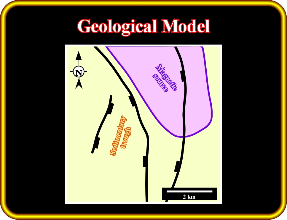
Plate 26.7 - As illustrated, a monocline geological model dipping westward with a small sedimentary trough, striking North-South and located in the western part of the map, is corroborated by the previous magnetic maps (Plates 8 to 12). Significant normal faults striking roughly north-south, seem to have lengthened the sediments. A magnetic source is likely in the north-eastern area. The proposed geological model must be tested by gravimetric and finally by seismic and subsurface data.
Summing up :
(i) Magnetic anomaly maps suggest the overall geological grain of an area, i.e, the orientation of basement highs and lows is generally apparent.
(ii) Faults may show up (close spacing or abrupt change of contours)
(iii) Sometimes, magnetic maps are used to differentiate basement (igneous and metamorphic rocks devoid of porosity) from the sedimentary cover that may be prospective. However, such a differentiation is just possible when there is a sharp contrast between the magnetic susceptibility of the basement and cover and where this contrast is laterally persistent.
(iv) Magnetic anomaly maps are also useful in petroleum exploration for indicating the presence of igneous plugs, intrusive rocks, or lava flows, i.e. areas normally avoided in the search for hydrocarbons.
(v) Seismically delineated “reef” have often been drilled and finally interpreted as igneous intrusions or volcanic plugs. A quick check of a magnetic map would indicate the presence of a magnetic anomaly and suggest an igneous intrusion rather than a reef.
In conclusion:
Magnetic surveys are a quick and cost effective way of defining broad basin architecture. Though, they can seldomly be used to located drillable petroleum prospects.
to continue press
![]()