The basis of the gravity method is the Law of Gravitation, which states that the force of attraction F between two masses m1 and m2, whose dimensions are small with respect to the distance r between them, is given by:
where G is the Gravitational Constant.
Considering the gravitational attraction of a spherical non-rotating, homogeneous Earth of mass M and a radius R on a small mass m on its surface, it is relatively simple to show that the mass of a sphere acts as though it was concentrated at the centre of the sphere. Using M, R and m on the previous equation, the force of attraction F is given by
Force is related to mass by acceleration and the term
. It is known as the gravitational acceleration or, simply, gravity.
- The mean value of gravity at the Earth‘s surface is about 9.80 m /s.
- Variations in gravity caused by density variations near earth's surface are expressed in micrometer per second (gu).
The gravitational field is most usefully defined in terms of gravitational potential:
U = GM/r
Whereas the gravitational acceleration g is a vector quantity, having both magnitude and direction (vertical downward), the gravitational potential U is scalar, having magnitude only. Small differences or distortions in that field from point to point over the surface of the Earth are caused by any lateral variation in the distribution of rocks in the Earth’s crust:
- If the Earth‘s subsurface was of uniform density (spherical non-rotating, homogeneous Earth of mass M), the Earth’s gravitational field, after the application of certain corrections, would everywhere be constant.
- Any lateral density variation associated with a change of subsurface geology results in a local deviation in the gravitational field. Geologic movements, as salt flowage or faulting, induce lateral density variations.
- Local deviations from the otherwise constant gravitational field are referred to as gravity anomalies.
A Bouguer anomaly is a gravity anomaly calculated after corrections for: (i) Latitude, (ii) Elevation, and (iii) Terrain
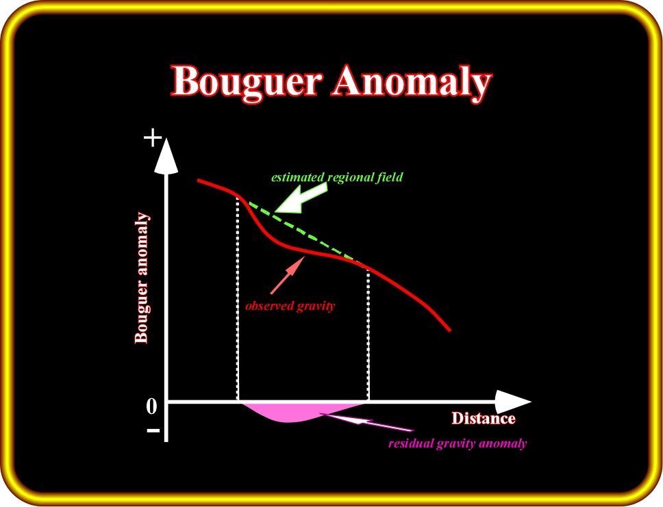
Plate 26.8 - The Bouguer anomaly (BA) corresponds roughly to the difference between the estimated regional gravity field and the observed gravity. In fact, this difference must be corrected by free-air correction (FAC), the Bouguer correction (BA), and the terrain correction (TC) or Eötvös correction (EC) when the gravity measurements are taken in a moving vehicle. Residual gravity anomalies are conventionally displayed on profiles or as isogal maps.
Regional and residual gravity anomalies must be individualized from the observed Bouguer anomaly:
(i) Bouguer anomaly fields (Plate 26.8 and 26.9) are often characterized by a broad, gently varying, regional anomaly on which may be superimposed higher wave number local anomalies, which are of prime interest in gravity surveying.
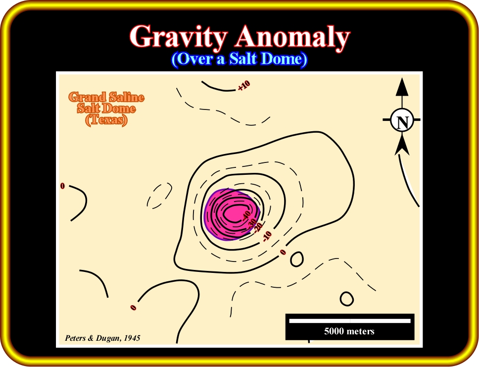
Plate 26.9- This map illustrates the negative gravity anomaly over the Grand Saline Salt Dome (see magnetic anomaly on Plate 7). The gravitational readings have been corrected for effects resulting from (i) Earth‘s rotation, (ii) Irregular surface relief and (iii) Regional geology. The contours reflect just variations in shallow density structures of the area induced by local geology. As depicted in Plate 6, the low density of the salt, generally between 2.15 and 2.17 g/cm3, induces a negative gravity anomaly.
(ii) The first step is the removal of the regional field to isolate the residual anomalies.
- Removal can be performed graphically by sketching in a linear or curvilinear field by hand.
- Graphic methods can be biased by the interpreter, but this is not necessarily disadvantageous as geological knowledge can be incorporated into the selection of the regional field.
- Several analytical methods of regional field analysis are available (trend surface analysis, low-pass filtering, etc.).
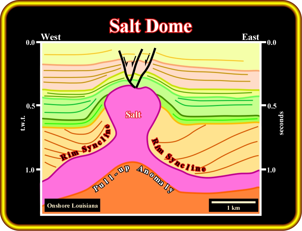
Plate 26.10- The magnetic and gravity anomalies illustrated on Plates 7 and 15 were performed over a salt dome that later was completely identified by this seismic line (Grand Saline Salt Dome, Texas, USA). Potential methods can roughly put in evidence the exact location and geometry of salt domes. They do not allow an exhaustive understanding of the geometry of the salt structures. Nevertheless, they can be used to test the coherence of the geological interpretations. In this particular example, the bulb and stem of the salt dome are quite evident as well as the associated rim synclines.
Gravity measured at a fixed location, varies with time because of periodic variation in the gravitational effects of the Sun and Moon associated with their orbital motions. Correction must be made for this variation in a high precision survey.
- Gravitational effects cause the shape of the solid Earth to vary in much the same way that the celestial attractions cause tides in the sea.
- Solid Earth tides are considerably smaller than oceanic tides and lag farther behind the lunar motion.
- Solid Earth tides cause the elevation of an observation point to be altered by a few centimeters and thus vary its distance from the center of mass of the Earth.
As with other geophysical methods, explorationists should not forget the epistemological limitation of gravimetry. Indeed, gravimetric, as well as magnetic methods are deterministic. Therefore, fundamentally
“an anomaly map corroborates or refutes a geological interpretation”
It is rare that a gravimetric map allows a direct accurate geological interpretation. Gravity is acceleration. Its measurement should simply involve determinations of length and time. However, the measurement of an absolute value of gravity is extremely difficult and requires complex apparatus and a lengthy period of observation.
The sequence of gravimetric data interpretation can be summarized as follows:
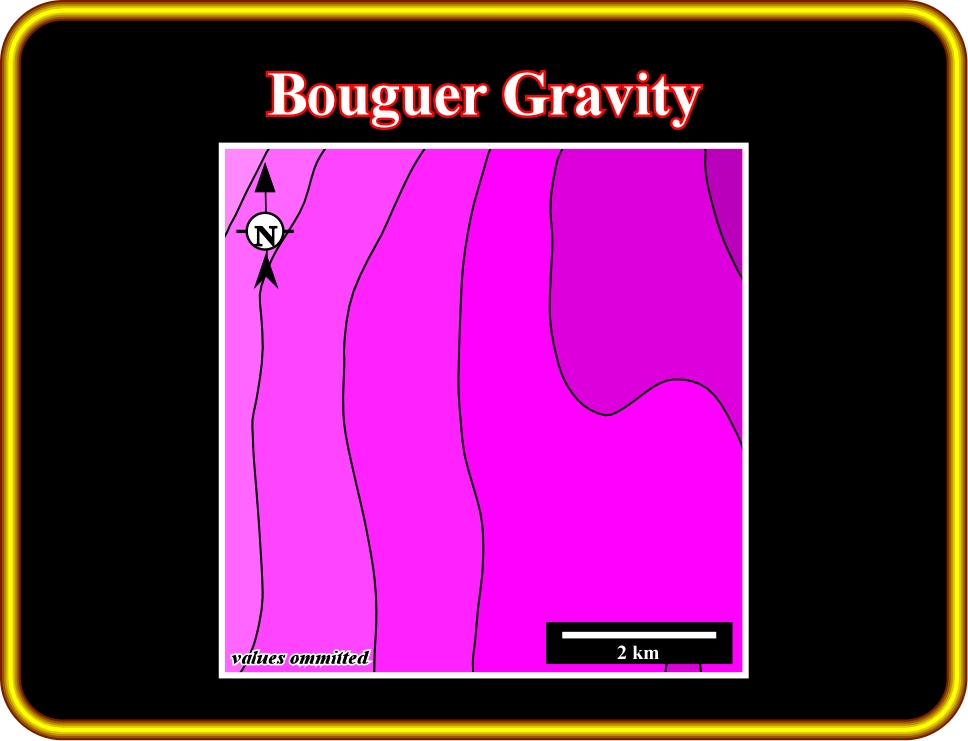
a) Bouguer Gravity
Plate 26.11- This map illustrates the Bouguer Gravity of the area covered by the magnetic anomaly depicted in Plate 26.2. It represents the gravity anomaly corrected for topographic and elevation effects.
Corrections for the differing elevations of the gravity stations is made in three parts:
1) Free-Air Correction (FAC)
It corrects the decrease in gravity with height in free air resulting from increased distance from the centre of the Earth, according to Newton's Law.
2) Bouguer Correction (BC)
It removes the gravitational effect of the rock present between the observation point and datum.
3) Terrain Correction (TC)
It takes into account the topographic relief in the vicinity of the gravity station. This correction is always positive.
b) Regional Gravity
The estimated regional field is calculated using the observed gravity as shown on Plate 26.8.
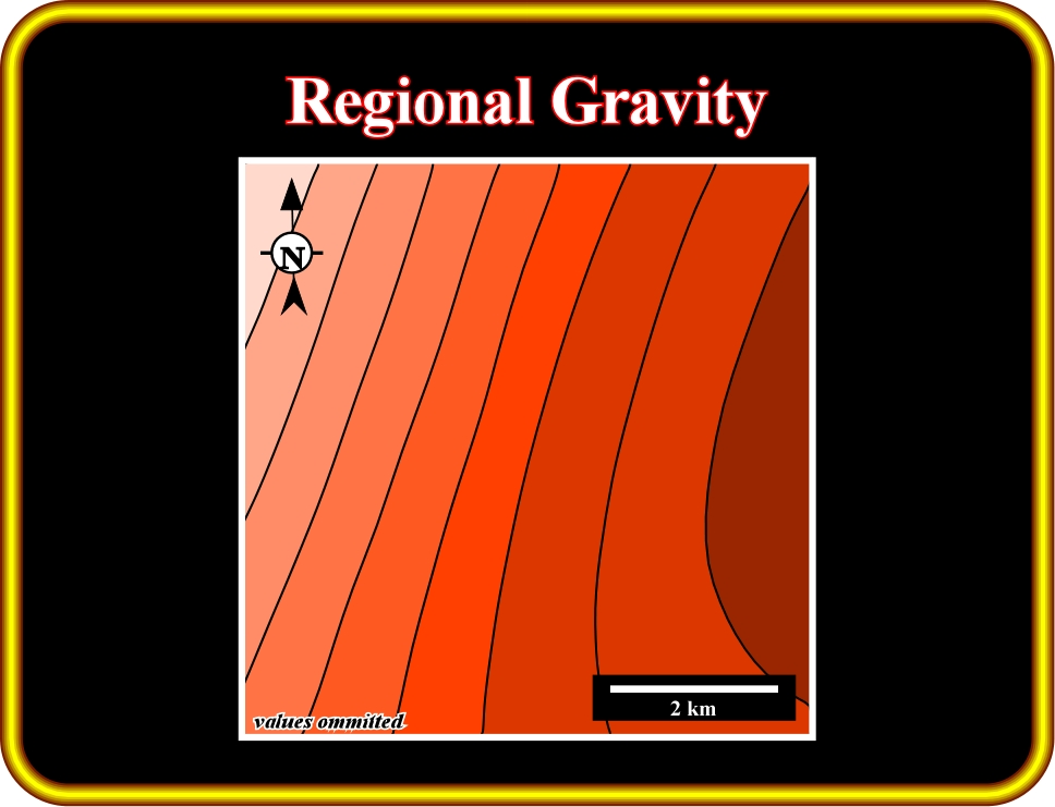
Plate 26.12- This map illustrates the Regional Gravity. It represents the long wavelength of the gravimetric anomaly associated with deeper sources.
c) Residual Gravity
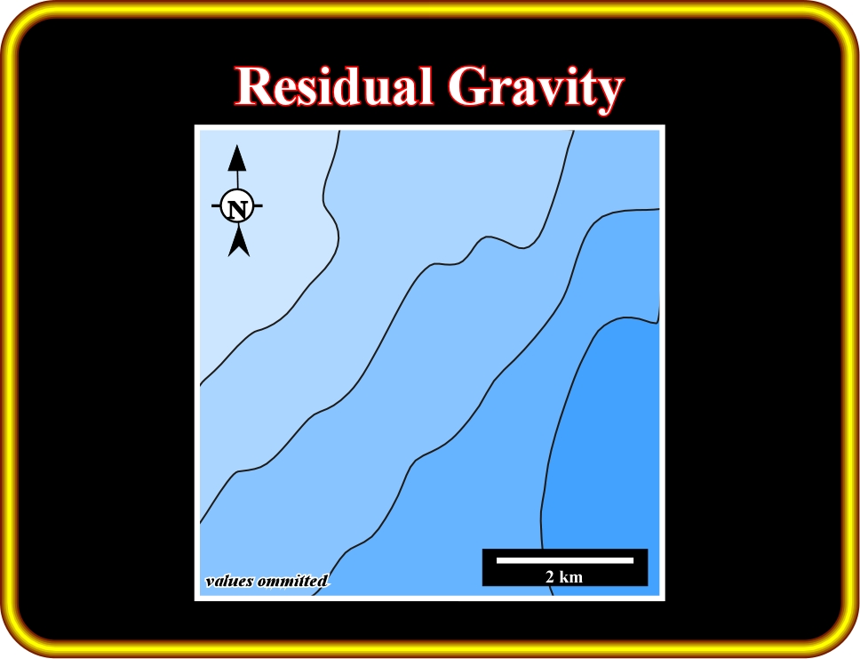
Plate 26.13 - This Residual Gravity represents the short wavelengths of the anomaly related to shallower sources. In other words, it represents the gravity anomalies when the regional field is removed.
To isolate the residual anomalies it is necessary to remove the regional field:
- This can be made graphically, but such a method is often biased by interpreters.
- Several analytical methods of regional field analysis are available and include trend surface analysis (fitting a polynomial to the observed data) and low-pass filtering.
d) Second Vertical Derivative (SVD) of Bouguer Gravity
As for magnetics, gravimetric anomalies can be enhanced by the second vertical derivative of Bouguer anomaly maps. These maps are necessary since limiting depth refers to the maximum depth at which the top of a body could lie and still produce an observed gravity anomaly.
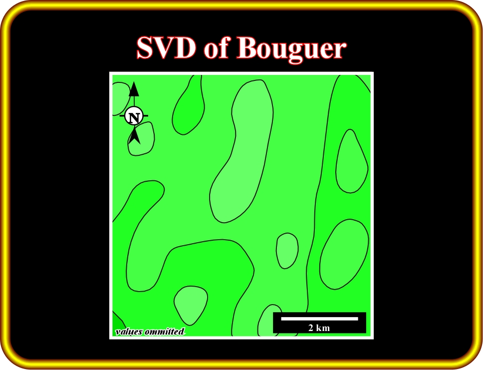
Plate 22.14- Here is illustrated the second vertical derivative map of Bouguer anomaly of the area covered by Plate 18. The enhancement induced by the derivative allows a better localization of the sources.
Actually,
- Gravity anomalies decay with the inverse square of the distance from their source.
- Anomalies caused by deep structures are of lower amplitude and greater extent than those caused by shallow sources.
- The waves number-amplitude relationship to depth may be quantified to compute the maximum depth at which the top of anomalous body could be situated.
e) Second Vertical Derivative (SVD) of Residual Gravity
As for Bouguer anomaly, the second vertical derivative map of the residual gravity can be quite useful.
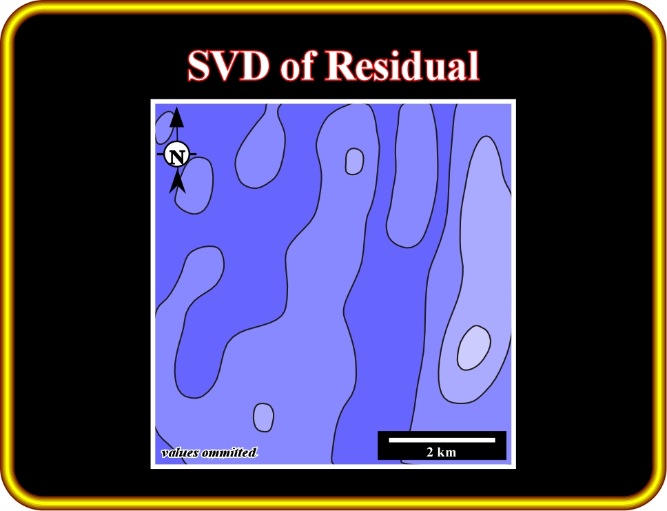
Plate 26.15- As for the Bouguer anomaly, the residual is here enhanced by the second derivative. The location of the gravimetric sources is more evident than in the residual map (Plate 26.13).
f) Gravity Interpretation
Gravity interpretation, as in magnetics, can be done by direct and inverse methods of interpretation. Direct interpretation provides, directly from the gravity anomalies, information on the anomalous body which are largely independent of the true shape of body. Various methods are used:
(i) Half-width method,
(ii) Gradient-amplitude ratio method,
(iii) Second derivative methods.
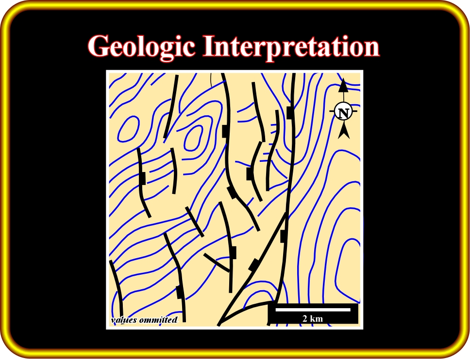
Plate 26.16- An extensional geological monocline, as illustrated above, fits with the gravimetric data (Plates 17 to 21). The area seems to be affected by an extensional tectonic regime characterized by a
1 (maximum effective stress) vertical and
In indirect or inverse interpretation, the causative body of a gravity anomaly is simulated by a model whose theoretical anomaly can be computed, and the shape of the model is altered until the computed anomaly closely matches the observed anomaly. Because of the inverse problem, this model will not be a unique interpretation, but ambiguity can be decreased by using other constraints on the nature and form of the anomalous body:
A simple approach to indirect interpretation is the comparison of the observed anomaly with the anomaly computed for certain standard geometrical shapes whose size, position, form and density contrast are altered to improve the fit.
Geological Models
1- Anticline Model
During a compressive tectonic regime (a horizontal
= 0.17 g/cm3 gives a typical antiform gravimetric anomaly (bottom of Plate 23).
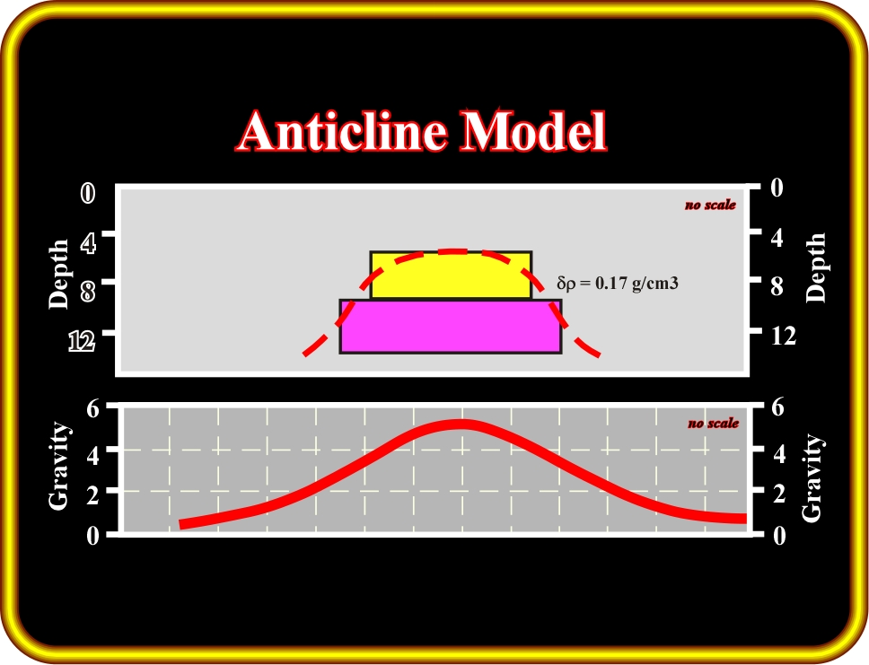
Plate 26.17- Geological model of an anticline structure and its gravity response with for a d
2- Thrusting Model
In a thrust or reverse fault, the sediments of the upthrown block (hangingwall) are shortened and uplifted, whereas those of the downthrown block (footwall) are relatively undeformed. In such conditions, as illustrated on Plate 26.18, the hangingwall sediments are denser than those of the downthrown block. In addition, as the hangingwall sediments are shortened, by folding, the structures’ heart is denser. The gravimetry response of such a geological structure is shown on Plate 26.18, where a strong positive anomaly correlates with the upthrown block.
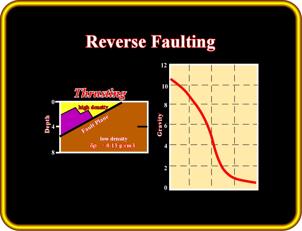
Plate 26.18- Geological model and gravity response for a thrust fault (or reverse fault), in which the density difference between the hangingwall and the footwall is d
3- Normal Faulting
During an extensional tectonic regime (a vertical
(i) Density and velocity of sediments of the downthrown blocks are higher than those of the upthrown blocks,
(ii) When the amplitude of the vertical throw is big enough, the associated lateral changes in density and velocity will create relatively important gravimetric anomalies.
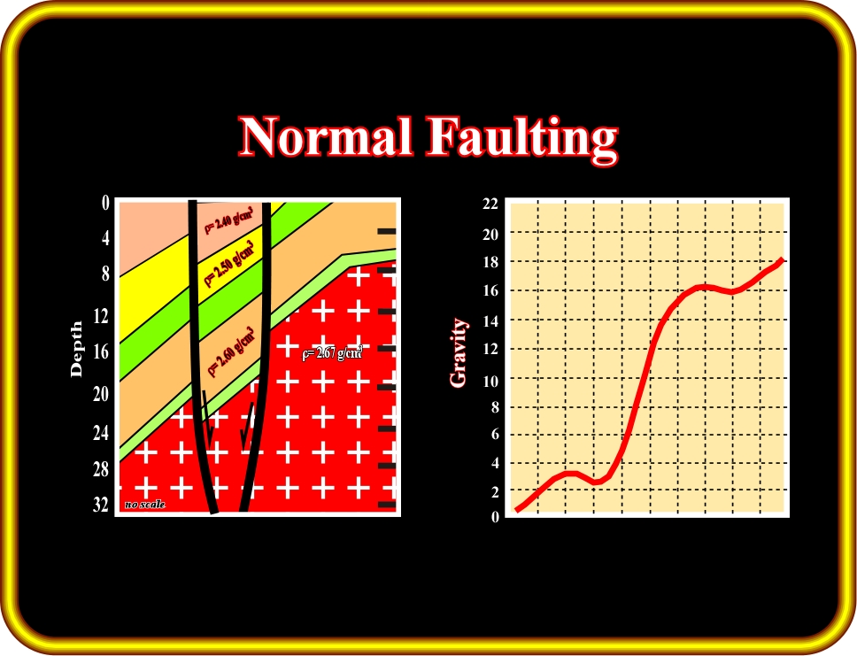
Fig. 26-19- In normal faulting, the hangingwall sediments are denser than the sediments of the upthrown block. Hence, as illustrated in the gravimetry profile, the associated gravimetric anomaly can be relatively sharp.
4- High Density Beds
In a geological model with high-density beds, the dips of the sedimentary beds can range from 10° to 60°. Assuming that sedimentary tilting is pre-compaction, there are lateral changes in density and velocity. Higher are the dips of the beds, the bigger are the lateral changes in density and velocity. Lateral contrasts are big enough to create sharp gravity anomalies, as illustrated below.
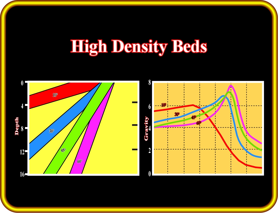
Plate 26.20 - On this geological model, the dips of the strata increase in depth. Hence, due to compaction, one can say that average density and acoustical impedance increase too. So, gravity anomalies can be associated with such a tectonic behavior.
In conclusion:
- Gravity maps are seldom used for detailed interpretation.
- Seismic surveys are generally more useful for detailed studies in small areas.
- Like magnetic, gravity maps are useful to show the broad architecture of sedimentary basins.
- In gravimetry, low-density depocenters appear as negative anomalies (salt domes, rim synclines).
- Buried hills of dense basement rock, in gravimetry, show up as positive anomalies.
to continue press
![]()