C- Interpretation Difficulties

When interpreting a seismic line, interpreters must take into account that (i) generally they work with time section and not with depth sections and (ii) artifacts should remain after or even could have been generated by seismic processing. Actually, if horizontal and vertical subsurface velocities were everywhere constant, a seismic line section would be the exact image of its underlying geological cross-section. However, under such conditions seismic profiles would show no reflections at all.

Fortunately, the real world is different :

- Firstly, ground compaction of stratigraphic layers under their own weight causes velocities to increase naturally with depth ;

The deeper the depth of burial of a geological level the faster is the velocity of propagation of the acoustic waves through it. One second (t.w.t.) of a shallow section, with a velocity of 2000 m/s, represents 1000 m of geological section. Hence, seismic time-sections are progressively squashed from top to bottom.

- Secondly, seismic velocities also depend on horizontal and vertical varying lithology. These variations are superimposed on the normal vertical distortion due to compaction.

The only way to view true scale seismic is to convert time-sections into depth sections. This implies a good understanding of the local velocity field and, the use of an iterative velocity model (as for depth migration).

C. 1) Time sections versus depth sections

In order to understand the difference between a time section (seismic line) and a depth section (geological cross section), let's consider a typical geological model taken from Kwanza basin (Angola) based on several wells’ results and field cross-sections (Plate 31).

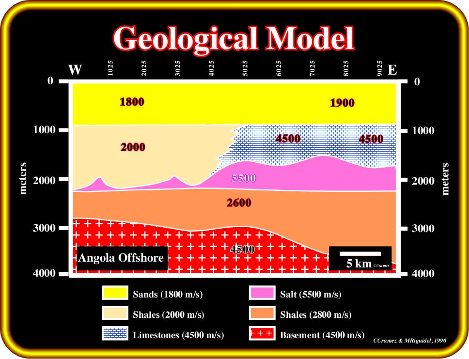
Plate 31- On this geological model, taken from Angola offshore, above the basement (which often corresponds to a Paleozoic fold belt) rift-type basins were developed during the rifting phase, preceding the breakup of the lithosphere (breakup of Gondwana). Overlying the breakup unconformity an Atlantic-type divergent margin was deposited. A more or less continuous salt layer and a limestone platform were deposited in the lower part of the divergent margin. Subsequently, lateral variations in velocity intervals are quite frequent, as illustrated above. Particularly interesting is the velocity change between the limestone platform (± 4500 m/s) and the coeval slope shales (± 2000 m/s), since it induces quite sharp artifacts in seismic lines (see next).

It is interesting to note that in this cross-section there are sharp lateral and vertical changes on the velocity of the seismic waves through the sediments :

- Through the sediments associated with rift-type basins, mainly organic rich shales and sandstones, the seismic waves travel at relatively low velocity ;

- Overlying the type-rift basin sediments, an evaporitic interval was deposited with a basal limit more or less horizontal showing significant thickness changes ;

- The seismic waves travel through the evaporitic interval with a high velocity (more or less 5500 m/s) ;

- Above the evaporitic interval, in the landward part of the section, limestones were deposited whereas, in the distal part, overpressured slope-shales overly the evaporitic layer ;

- Finally, in the upper part of the section, an undercompacted shale-sand interval characterized by a velocity interval ranging between 1800-1900 m/s was deposited ;

- Briefly, the velocity of the seismic waves through these facies (lithologies and not environments) are quite different as indicated in Plate 31 (4500 m/s, 2600 m/s, 5500 m/s, 2000 m/s and 1800 m/s). Through the sediments of the type-rift basin, mainly organic lacustrine shales and sandstones, the seismic waves travel at relatively low velocity.

The seismic synthetic response of this geological model is illustrated in Plate 32. It depicts the difference between a geological cross-section (depth section) and a seismic line (time section).

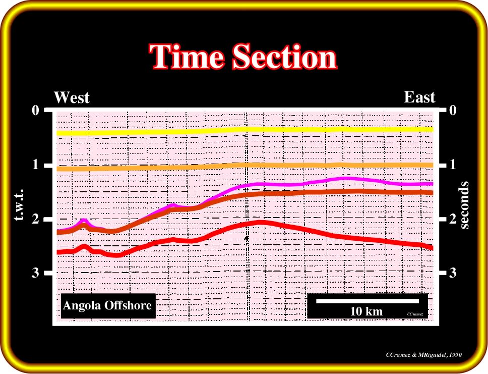
Plate 32- This time section is the synthetic seismic response (time section) of the geological model illustrated on Plate 31. The red marker corresponds to the interface basement / sediments, that is to say, the top of the basement (granite-gneiss or more or pre-Pangea sediments). However, it does not correspond to a real chronostratigraphic line, but to an unconformity, i.e., an erosional surface induced by a significant relative sea level fall. The brown marker fits with the bottom of the evaporitic interval, while the violet marker emphasizes the top of the evaporites. The light brown and the yellow markers correlate with the bottom and top of the undercompacted shale/sand interval. The pull-up of the horizon emphasizing the bottom of evaporites (brown marker) is a consequence of the high velocity of the seismic waves through the salt interval. The interval, between the violet and brown markers, corresponds to the limestone platform and slope shales. The high velocity of the seismic waves in the limestones is the responsible for its small time-thickness (eastern part of the time section). In contrast, the low velocity of the seismic waves through slope shales explains their large time-thickness (western part of the violet/brown interval). The majority of geoscientists working in petroleum exploration define a pull-up (Schlumberger Oilfield Glossary) as a phenomenon of relative seismic velocities of strata whereby a shallow layer or feature with a high seismic velocity (e.g., a salt layer or salt dome, or a carbonate reef) surrounded by rock with a lower seismic velocity causes what appears to be a structural high beneath it. After such features are correctly converted from time to depth, the apparent structural high is generally reduced in magnitude.

Indeed:

a) Similar interval time thicknesses can correspond to quite different interval depth thicknesses ;

b ) Interval depth thickness is dependent of the velocity of the seismic waves through each interval ;

c) The geometry of the boundaries of the different sedimentary packages are quite different ;

c) In time, the base of the evaporitic interval is not horizontal, as in the geological model, but strongly deformed by the lateral velocity changes ;

d) The top of the basement shows an antiform geometry under the change of facies from limestones  to shales.

Let's see some real examples:

Example n° 1 (Plate 33)

This example comes from the west Palawan offshore (Philippines), where, in the 70’s, several oil companies explored the conventional offshore (water depth less than 200 m) :

(i) An exploration well was supposed to test the hydrocarbon potential of a structural high ;

(ii) The structural high was identified on unmigrated seismic lines ;

(iii) The original seismic line, where the well was located, is illustrated in the upper part of Plate 33 ;

(iv) On the seismic line (time), the structural high is located directly above the present limit between continental shelf (less than 200 meters water depth) and the upper slope environment, that is to say, above of  an abrupt change of the water depth (bathymetry) ;

(v) The structural high was interpreted as a potential reef anomaly located nearby a shelf break (the depositional coastal break is far away landward of the shelf break since the basin, at that time, as today, had a significant continental platform defined between zero and 2oo meters of water depth) ;

(vi) The exploratory well was drilled and suspended around 200 meters below the apex of the structural high of the potential reservoir-rock (upper part of Plate 33).

(vii) The results of the well were negative. In fact, no indications of hydrocarbons and no reservoir-rocks were recognized.

After the negative results of the well, a depth-migration of few seismic lines was performed. A depth-time conversion of the line where the wildcat was located is illustrated in the lower part of Plate 33 (the vertical scale is in feet and not in t.w.t.).

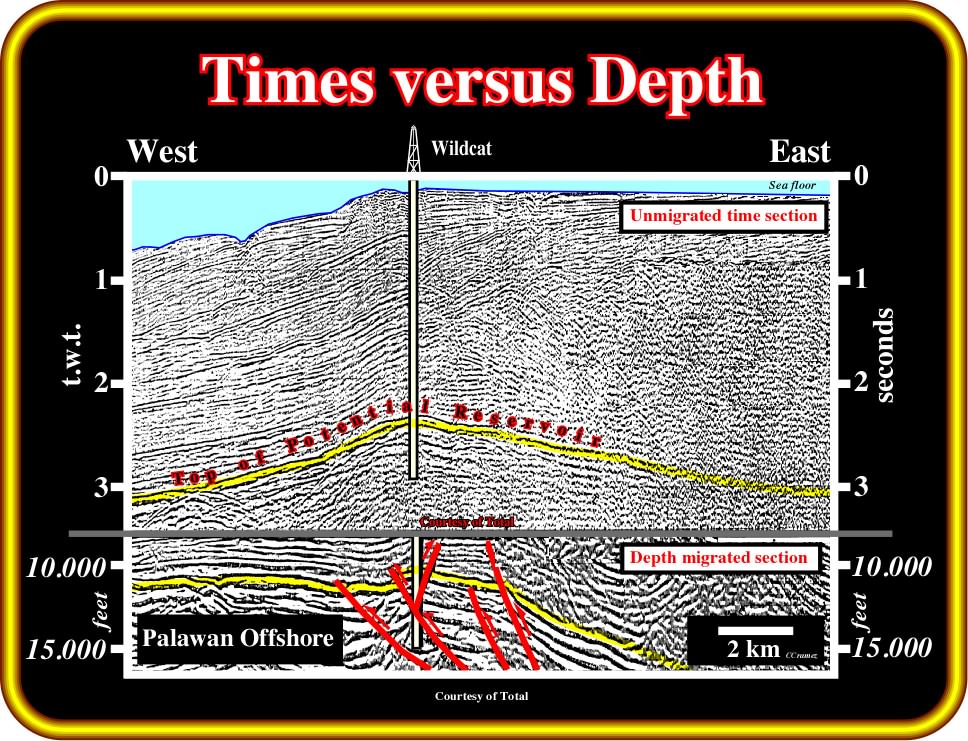
Plate 33 - In the upper part, an unmigrated time version of a seismic line, where an exploratory well was located, is illustrated. In the lower part, is shown the depth migrated version of the potential revervoir interval. The depth version strongly suggests that the time-structural high corresponds to a seismic artifact and not to a real antiform structure (extensional structure created by lengthening of the sediments and not by shortening). In other words, the prospect is not a structural trap, but a morphological trap by juxtaposition. The geoscientists in charge of the evaluation of such a lead (trap which may contain hydrocarbons) not only forgot that the west Palawan offshore is located within the Meso-Cenozoic megasuture, that is to say, located in a compressional geological setting, but also they did not take into account that an abrupt increasing in the water-depth induces a significant pull-down (opposite of a pull-up) of the seismic horizons located below the present shelf break (limit between the continental platform and continental slope).

Comparing the two seismic versions, geoscientists readily understood:

The time-structural high corresponds to a seismic artifact induced by the abrupt water depth and facies change in the sediments overlying the potential reservoir-rock.

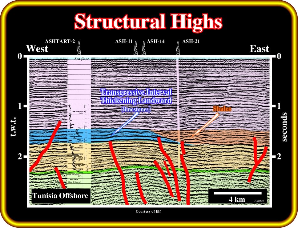
Example n° 2 (Plate 34)

This example comes from the offshore Tunisia. It illustrates what interpreters should not do when assessing expected producing reserves in an oil or gas accumulation. In other words, geoscientists should never forget :

a) The difference between a seismic line and a geological cross section :

- A seismic line corresponds to a time-profile (the vertical scale is in time and the horizontal scale in meters) ;

- A geological cross section is a depth-profile (the vertical and horizontal scales are in meters) with or without vertical exaggeration ;

b) All tentative geological interpretations of a seismic line must be tested (criticized) :

- The more coherent and realistic tentative interpretation is not the nicest, but the more difficult to refute.

The philosophy of geological tentative seismic interpretation, as well as, other geological interpretations, can be summarized as follows :

(i) At the beginning, geoscientists have a problem (e.g., find hydrocarbons) ;

(ii) In order to solve the problem, they must propose or advance an hypothesis (tentative interpretation), what implies a certain a priori geological knowledge ;

(iii) Then, they must try to refute the advanced hypothesis. Such refutation test can be done with new or old observed data (drilling, new seismic, etc.) ;

(iv) Arriving at this point, two possibilities can be considered:

a) The refutation test failed. Hence, with the available data, the tentative interpretation can be considered as probable, that is to say, the hypothesis is corroborated by the available data, but it is not true. New data can refute it (there is no true seismic interpretation) ;

b) The interpretation is refuted. In this case, the geoscientist gets a new problem, which implies a changing of the initial hypothesis. A new hypothesis (new tentative interpretation) must be advanced, which afterward must be tested and so on.

This scientific approach by trials and errors is the best way to make substantial progress in geological sciences, seismic interpretation and petroleum exploration.

In this example (Plate 34), the same seismic pitfall (an unforeseen or unexpected or surprising seismic difficulty), which can be reported as follows:

On time seismic profiles with lateral changes in velocity interval, the highest time-structural point of a seismic marker does not necessary correspond to the highest depth-structural point.

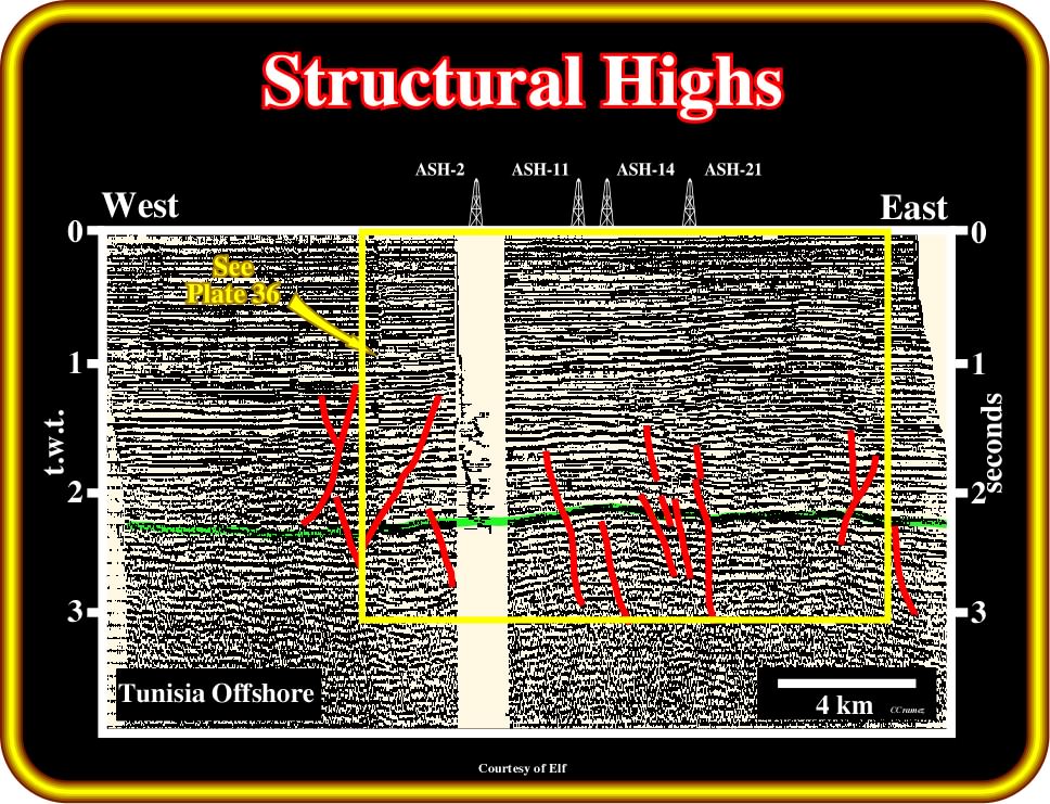
Plate 34- Take note that this seismic line comes from Tunisia offshore, that is to say, from an area located inside of the Meso-Cenozoic megasuture (record of folding, thrust faulting and igneous activity). In addition, the lengthening of the Pangea sediments seems to have been big enough to breakup the lithosphere creating a marginal sea (oceanization). Briefly speaking, the basin setting is that of Mediterranean-type basin (globally compressional). On this line (time section), it is easy to recognize that the highest time structural point along the picked reflection (green marker) is near the well ASH-11. However, as shown later (Plate 36) due to lateral facies and velocity changes, this time structural point does not correspond to the highest depth structural point.

On a time-seismic line (from now on, on these notes, a seismic line expresses a time-seismic profile) not all time-structural high points correspond to depth-structural high points. Geoscientists in charge of Tunisia offshore, using untested tentative geological interpretations of the seismic lines, proposed to their management time contour maps of the top of the potential reservoir (green marker on Plate 35), in which a small structural closure was visible. The management (those in charge of running a business) decided to test such a play (a particular combination of reservoir-rock, seal-rock, source-rock and trap associated with proven hydrocarbon accumulations). The results of the well were positive, i.e., hydrocarbons were found on the predicted reservoirs-rocks.

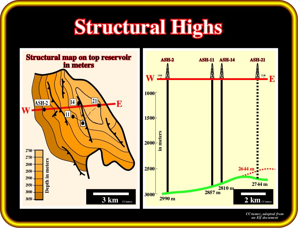
Plate 35- Before the drilling of well ASH-21, the depth contour maps of the field were similar to the one illustrated on the left part of this plate and the structural sections of the reservoir-rock (in green) similar to the one illustrated on the right. The highest structural point was located westward of ASH-14, eastward of the proposed location of ASH-21. However, the results ASH-21 indicated the actual highest depth point was located westward of ASH-21, at 2644 m (in red). These results completely refute the proposed time geologic interpretations of the field, which, by the way, were mainly based in the picking of the top of the reservoir interval. As shown next, it seems that the geoscientists, in charge of the development of the field, forget that a single naive tentative interpretation (picking in continuity just one marker) must fit within the global geological picture. In Geology, and particular in Petroleum Geology (Petroleum Systems), geoscientists progress from the general to the particular and not from the particular to the general.

After drilling, explorationists took the positive results as a verification of their tentative geological interpretations of the seismic lines. Such an attitude is highly dangerous (verificationism) and the consequences can be catastrophic. In fact, a geological interpretation can never be verified (in Latin verus means true). As said previously, true geological interpretations do not exist :

- The verification of a tentative geological interpretation is impossible ;

- Data can corroborated or validated tentative interpretations ;

- Corroboration, Validation and Verification are not synonyms ;

- New data can always refute a previous corroborated interpretation.

Following this erroneous attitude, several wells were proposed and drilled with successful results and a development phase took place. At that time (before the drilling of ASH-21), the structural sketch of the field at the reservoir level, assumed by the geoscientists, was similar to that illustrated in Plate 35.

Actually:

- Before the drilling of ASH-21, the converted seismic depth map, calibrated with the results of the wells (Plate 35), indicated the highest structural point slightly (800-1000 m) eastward of ASH-14, as shown in the W-E cross section (green marker) ;

- The well ASH-21 was proposed and the forecast depth of the top of the reservoir-interval was at 2744 meters ;

- After the drilling of ASH-21, surprisingly, the top of the reservoir-interval was found 100 meters higher and the apex of the structure was not located 800-1000 m westward of ASH-14 (± 1000 m westward of the well ASH-21).

The substantial increasing of the hydrocarbon “reserves” following the drilling of ASH-21 masked the mistake made by the seismic interpreters (all reserve estimates involve uncertainty, depending on the amount of reliable geologic and engineering data available and the interpretation of those data). Nevertheless, the understanding of the surprising results of well ASH-21 became extremely important in order to avoid future mistakes. The interpreters forgot that a seismic line is a time section and not a depth section. Lateral lithological changes, above the reservoir-rock, must be taken into account during the interpretation, since they induce lateral velocity changes, which, in a depth section, can invert the relative position between two points:

In a time section, function of the interval velocities, a relatively high structural point can become a relatively low point, in a depth converted section.

Plate 36- This line corresponds just to an enlargement of the line illustrated on Plate 34. It shows a transgressive backstepping-interval thinning seaward (in green). Such a thinning creates a lateral change in facies and so, in velocity interval. The different time-thickness of this transgressive calcareous interval, drilled in ASH-2 and ASH-21, readily explains why the highest time-structural point of the potential reservoir (lower green marker) does not match with the highest depth-structural point: the seismic waves do not travel at the same velocity in limestones and slope shales. The markers below the slope shales are pulled-down.

A geological tentative interpretation in sedimentary packages and not just following single and more or less continuous reflections of the seismic line (Plate 34) strongly suggests a sedimentary interval between 1.5 and 1.75 seconds (t.w.t.) in the left part of the line (colored in blue on Plate 36):

- This sedimentary package thins rigthward and becomes very condensed near the location of ASH-21 ;

- Such a geometry is associated with a transgressive episode, in which deposits thicken landward as the depositional coastal break backsteps and the water depth increases creating a larger shelf (continental platform).

In fact, it is easy to recognize a lateral facies change:

- Seaward of the Oligo-Miocene shelf break (abrupt dip change in the blue interval), the limestone platform thin gradually seaward (actually it backsteps) ;

- The backstepping geometry of the transgressive limestones is fossilized by shales, which creates a lateral diachronic facies change ;

- This change in facies induces a seaward slowing of the interval velocity ;

- Below the condensed backstepping limestones, near the ASH-21, seismic waves are delayed and the associated reflections (time) are pulled-down relative to those underlying the thick limestone package in the central and right part of the seismic line, which are pulled-up.

C. 2) Unmigrated versus Migrated Profiles

Multifold covered data display implies a geometrical approximation (Plate 37):

Source and receiver positions are removed artificially and placed on a same location by applying dynamic (or move out) correction.

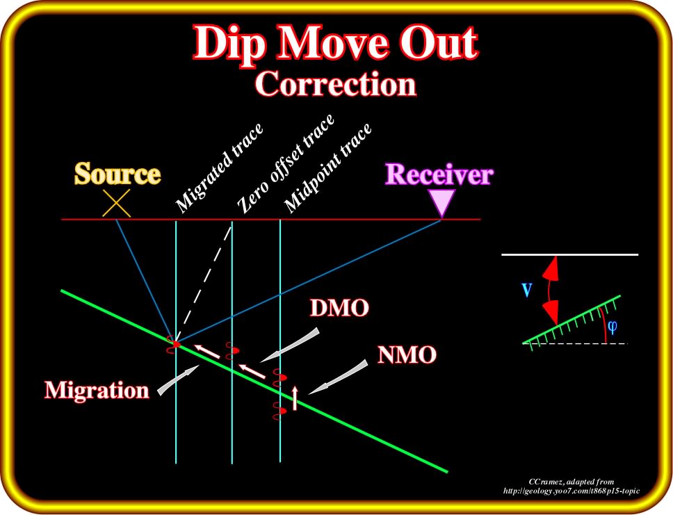
Plate 37- A function of time and offset that can be used in seismic processing to compensate for the effects of normal moveout, or the delay in reflection arrival times when geophones and shot points are offset from each other. Dip move out may be used to compute the reflector dip if V (average velocity) is known. V can be derived by a mathematical equation using the NMO (normal move out, that is to say, the difference between the travel times t1 and t2 of reflected ray arrivals recorded at two offset distance x1 and x2), which for small dips may be obtained with sufficient accuracy by averaging the up-dip and down dip move-outs.

- When a reflector is tilted, the reflectors paths arriving at two receivers, located at equal offsets up-dip and down-dip from a central shot point, are of different length. The rays will therefore have different travel times.

- Dip move out, which ensures non zero offset to zero offset conversion in the absence of dipping layers, is defined as the difference in travel times tx and t-x of rays reflected from the dipping interface to receivers at equal and opposite offsets x and -x.

- The steeper a reflector is the greater is its dislocation on an unmigrated time section.

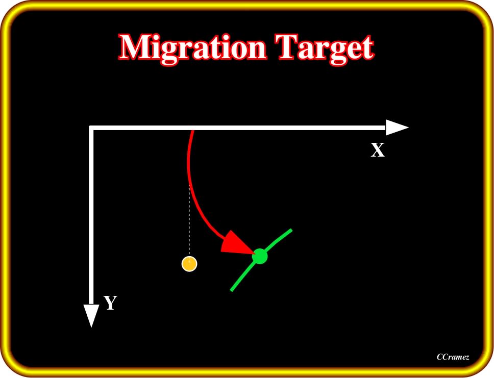
Migration (Plate 38) is the process of reconstructing a seismic section, in which reflection events are repositioned under their correct surface location and at a corrected vertical reflection time. In order to accurately migrate a seismic section, it would be necessary to define fully the velocity field of the ground, that is to say, to specify the value of velocity at all points. In practice, for the purposes of migration, an estimate of the velocity field is made from prior analysis of the unmigrated seismic section, together with information from borehole logs.

Plate 38 - Seismic migration is the process by which seismic events are geometrically re-located in either space or time to the location the event occurred in the subsurface rather than the location that it was recorded at the surface, thereby creating a more accurate image of the subsurface. This process is necessary to overcome the limitations of geophysical methods imposed by areas of complex geology, such as: faults, salt bodies, folding, etc. (http://en.wikipedia.org/wiki/Seismic_migration). For a given reflection time, the reflection point may lie anywhere on the arc of a circle centered on the source-detection position. On an unmigrated seismic section, the point is mapped to lie immediately below the source-detector. In a migrated line the point is repositioned under its correct surface location and at a corrected vertical reflection time.

Migration improves, also, the resolution of seismic sections by focusing energy spread over a Fresnel zone (one of a number of concentric ellipsoids resulting from diffraction by the circular aperture, which define volumes in the radiation pattern) and by collapsing diffraction patterns produced by point reflectors and faulted beds. By the same token, migration removes the diffracted arrivals resulting from point sources, since every different arrival is migrated back to the position of the point source.

Although, nowadays, the majority of the seismic lines used in petroleum exploration are migrated lines, it is interesting to make a review of the major differences between migrated and unmigrated data in order to understand not only the evolution of geological interpretation of seismic profiles, but the organization of the exploration teams as well.

A) Antiform Structures in Unmigrated Seismic Lines

Since a seismic section (unmigrated) presents its trace vertically below the observation point, it is evident that the seismic line will portray antiform structures a little wider than in the ground (Plate 39). In other words, the flanks of the structures are less steep. However, the crest of the structure is always in its correct positions with respect to the surface. Hence, crestal areas, with their low dips, are the least distorted areas.

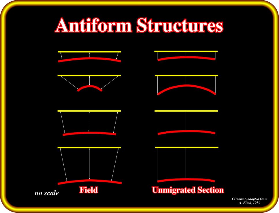
Plate 39 - These sketches illustrate the seismic responses of antiform structures with different geometries. It is easily to notice that on unmigrated seismic lines the closed surface associated to antiform traps is always overestimated. The term antiform (anticline or rollover) is here used in a descriptive sense and not genetic. Indeed, in the 70‘s, before the migration advent, the misunderstanding of this important feature could have catastrophic consequences. I remember quite well, as the majority of the large and apparently economic prospects (a prospect is lead which has been fully evaluated and is ready to drill) of Labrador Sea (based in unmigrated data) disappeared, as the first migrated versions of the seismic lines were performed.

The seismic answers of real earth antiform structures, such as anticlines (compressional or shortening structures) and rollovers (extensional or lengthening structures) on unmigrated seismic lines (Plate 39 ) were summarized as follows (A. Fitch, 1979):

(i) A gentle antiform is scarcely changed in its seismic expression ;

(ii) A sharply folded and narrow antiform may have seismic expression as a gently folded, wide antiform ;

(iii) The antiform will show less relief on the seismic response ;

(iv) A given antiform shape will have a wider seismic expression the deeper it gets ;

(v) Concentric anticline folds are parallel folds on seismic lines ;

(vi) Widening in depth of parallel folds can progress to the point where neighboring anticline folds can overlap in their seismic expression.

B) Synform Structures in Unmigrated Seismic Lines

Gentle synforms present few problems (Plate 40). Synforms become a little narrower on seismic than they are in fact. The lower point of the synform is undisturbed.

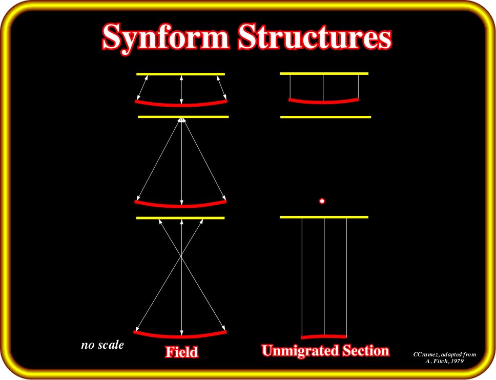
Plate 40- The illustrated relationships can be stated in terms of the position of the centre of curvature of a cylindrical real synform (field) : (i) when the centre of curvature is above the surface, the synform response is concave upward ; (ii) when the centre of curvature is at surface, the response is a point and (iii) when the center of curvature is in the subsurface, the synform response is convex upward.

A. Fitch (1979) summarized the seismic response (Plate 40) of a concentrically synforms (in parallel or concentric fold, the orthogonal thickness reamining constant along individual folded layers) as follows :

- Concentric synforms appear as parallel folds in the seismic response ;

- With parallel folding in the real earth, the deeper the synform reflector considered the narrower its seismic response ;

- A depth is reached, eventually, at which the seismic response of the whole synform is a single bright point. Below this level, the normal to deepest part of the synform is shorter than the normal to any point on the flanks of the synform, that is to say, the seismic response of such synform is convex upward, that means it looks like an antiform at first glance.

C) Complex Structures in Unmigrated Seismic Lines

Compression and intrusive bodies create complex structures that have seismic responses often difficult to interpret (Plate 41). The intrusive material may be : salt, mobile shale or volcanic. As, in many cases, sedimentary beds are strongly deformed around the top of the intrusive body. Droopy hyperbolas obscure the flank structures deeper down.

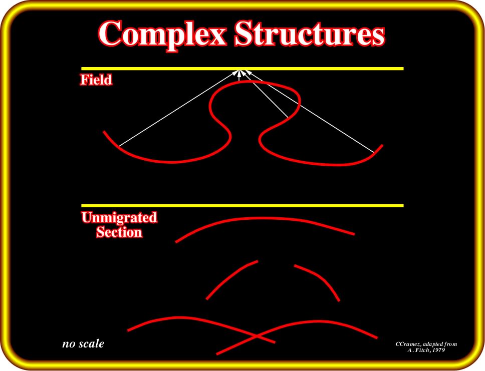
Plate 41- This sketch illustrated how complex is the answer of complex structures, here a salt dome (antiform) and its associated rim synclines (synforms), in an unmigrated seismic line. This complex answer was probably the main reason why before the advent of migration, the majority of the geoscientists in charge of the interpretation of seismic lines were primarily geophysicists with a good geophysical background, but, often, with a defective geological background.

In most cases, intrusive bodies have a piercement relationship, hence sedimentary beds, which are cut across, show typical fault features. Salt domes, being usually flanked by rim synclines, form very complex structures, which yield seismic responses that, at first, seem unrecognizable.

to continue press