
Universidade Fernando Pessoa
Porto, Portugal
Seismic-Sequential Stratigraphy
During my petroleum exploration career and academic activities, I have noticed that the approach to major problems in Earth sciences, and particularly the geological interpretation of seismic lines, is still dependent on Bacon’s heritage. Indeed, Bacon (Novun Organum, 1620) strongly suggested the scientific approach in natural sciences should be inductive. He considered Induction as the demarcation criteria between science and pseudo-science, theology or metaphysics.
“Scientific theories, or hypotheses,
should be established and justified by repeated observations”
In spite of the fact that J. Liebig (1985) and K. Popper (1934) criticize and partially rejected the use of inductive method on Natural Sciences, this approach still is strongly anchored in several oil companies. A lot of explorationists are still convinced they can make coherent and appropriate geological interpretations of seismic profiles without knowing Geology. Nevertheless, it is easy to show that seismic lines, such as the one, which interpretation is illustrated on Plate 1, can only be correctly interpreted, in geological terms, when the interpreter knows the geology of the area where the line was shot.
Actually, “Theory precedes Observation” (K. Popper, 1934), that is to say, an explorationist can only recognize on a seismic line, in the field, or on an electric log, what he knows. If he does not know what a thrust-fault, or an incised valley is, he can spend weeks looking at one or several seismic lines or outcrops, but the final result will always be the same:
“a geometrical description of more or less continuous, and well visible, reflections, or bedding planes, without understanding how they fit in the regional and global setting”
Indeed, when a seismic line is shown to:
a) An explorationist trained in seismic processing, he will see, besides the major reflections, multiples, diffractions, and coherent or incoherent noise patterns, etc.
b) An explorationist trained in structural geology, he will see faulted blocks, growth-faults, anticlines, overthrusts, etc.
c) An explorationist, trained in depositional processes, he will see prograding shelf edges, channels, submarine fans, etc.
d) An explorationist familiar with episodic depositional concepts, he will see turbidites, point bars, tidal deposits, shoreface sands, etc.
e) An explorationist, knowing the basic eustatic concepts, he will see stratigraphic-cycles, eventually sequence-cycles, downward shifts of coastal onlaps, lowstand deposits, highstand deposits etc.
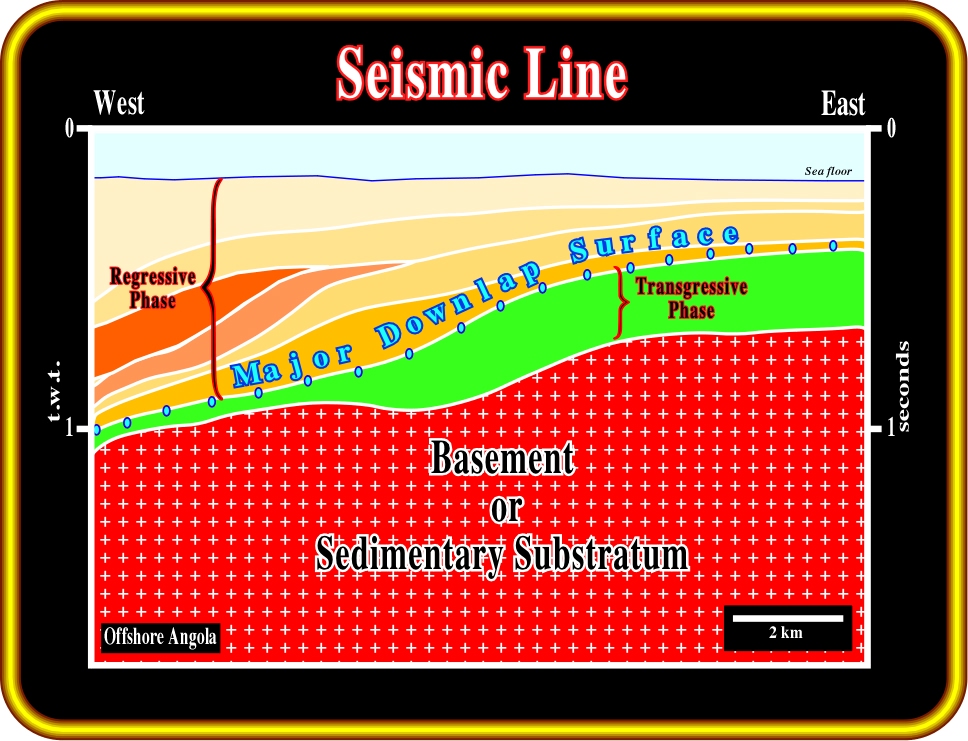
Plate 1- This interpretation of a seismic line, shot on the conventional offshore (< 200m) of Angola, pictures the proximal area of the Kwanza basin. This offshore is composed by the stacking of different sedimentary basins. The infrastructure is either a Precambrian granitic basement or a sedimentary substratum (Precambrian foldbelt or Karoo). The basement outcrops a few kilometers eastward with a granitic facies (gneiss with garnets). It is overlaid by Upper Jurassic / Lower Cretaceous rift-type basins (not present on this line) and a Meso-Cenozoic Atlantic-type divergent margin. The margin is composed by a transgressive and regressive phases. The transgressive phase has a backstepping geometry, while the regressive phase has a forestepping geometry. Hence, the interface between the transgressive and regressive phases corresponds to a major downlap surface. However, as illustrated, near the borders of the basin, the boundary between these sedimentary phases of the post-Pangea continental encroachment stratigraphic cycle is quite subtle. Several unconformities, associated with relative sea level falls, can be recognized, particularly in the regressive phase. That note that due to reasons of confidentiality, in the majority of the cases, only the interpretation of the seismic lines is illustrated. Nevertheless, the uninterpreted seismic lines are show during the short course.
If you think I am exaggerating, you can make a quick test using the sketch illustrated on Plate 2, which depicts a potential stratigraphic model of the Mahakam offshore (Indonesia), in which the more or less continuous seismic reflections (chronostratigraphic lines) were taken from several seismic lines of the area.
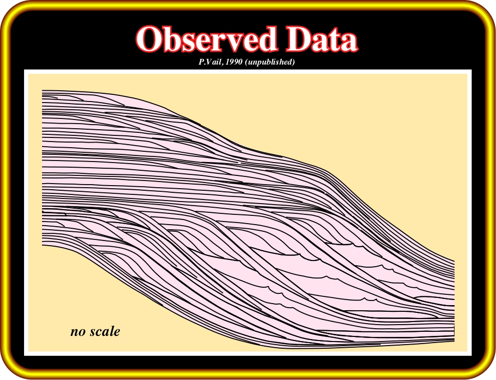
Plate 2- On this sketch, more or less continuous seismic reflectors, taken from several seismic lines shot on the offshore Kalimantan, in East Indonesia (Mahakam delta), are illustrated. Knowing the global and regional geological settings of this area (non-Atlantic divergent margin, in Bally's basin classification), the major stratigraphic events can be recognized using the geometrical relationships between the reflection terminations (see Plate 3). All sediments represent in the model were deposited during oceanization, that is to say, after the breakup of the lithosphere and subsequent formation of new oceanic crust (Non-Atlantic divergent margin above a backarc basin).
So, what do you see in the sketch depicted on Plate 2? In fact, if you are trained in sequential stratigraphy, it is possible that you recognized something similar to what is illustrated on Plate 3. In other words:
a) The cyclicity of the data.
b) The downward shifts of coastal onlaps.
c) The sequence-cycle boundaries (associated with 3rd order eustatic cycles).
d) The lowstand and highstand deposits.
e) The regression/transgression cycles (Genetical Stratigraphy);
f) The maximum flooding surfaces.
g) The most likely location of the potential source-rocks.
h) The most likely location of the potential sandstone reservoir-rocks.
i) The most likely location of the potential seal-rocks.
j) The most likely potential of the potential stratigraphic traps, etc.
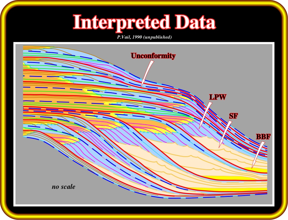
Plate 3- This figure depicts the observed data recorded by an explorationist trained in sequential stratigraphy and knowing the global and regional geological settings of the area where the seismic line was shot. He recognized several relative sea level falls (RSLF) and the associated unconformities (sequence-cycle boundaries), in red, as well as, highstand and lowstand depositional systems. Seaward of the shelf-breaks, he identified basin floor fans (BFF), slope fans (SF) and lowstand prograding wedges (LPW). Similarly, he recognized intervals during which progradation was dominant (regressions) and those where retrogradation (transgressions) was paramount.
Probably, you will propose a final interpretation similar to that illustrate on Plate 4, in which the sedimentary driving concepts controlling deposition:
(i) Sequential Stratigraphy
(ii) Eustatic Cycles
were taken into account in the interpretation.
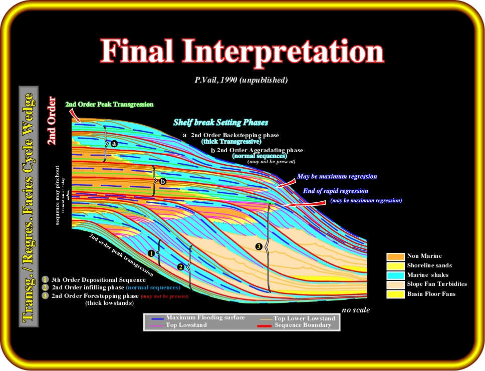
Plate 4- The observed data (see Plate 2) can finally be interpreted in terms of sequential stratigraphy. The interpreter took into account not only the driving concepts of sequential stratigraphy and eustasy, but also the global and regional geological settings of the area. In spite of the fact that in this example tectonic knowledge is not required, it must be pointed out that a significant knowledge in Tectonics is also indispensable to perform coherent and realistic seismic interpretations, i.e., interpretations difficult to refute. In fact, Geology is holistic. Its parts, such Stratigraphy, Sedimentology, Tectonics, etc., are interlinked and interconnected.
Summing up:I may indeed be wrong, but I strongly think explorationists see what they know and what they have been trained to see. When making observations, particularly on seismic data, it is necessary to understand the driving concepts controlling observations. Seismic interpreters must critically test their interpretations, present them to others, and listen to what they say. The same basic principles apply to the interpretation of the electric-log and outcrop.
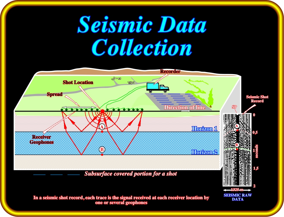
According to Nettleton (1976), any conceivable property or process, which can be measured or carried out at above the surface, and, which is affected by the nature of rocks through a cover of hundreds to many thousands of feet of intervening rocks, may be made the basis of a method of geophysical prospecting. Fundamentally, there are two main families of geophysical surveying (P. Kearey and M. Brooks, 1993):
(i) Natural Field Methods
They utilize the gravitational, magnetic, electrical and electromagnetic fields of the Earth. They look for local perturbation in these naturally occurring fields that may be caused by concealed geological features.
(ii) Artificial Field Methods
They involved the generation of local electrical or electromagnetic fields that may be used analogously to natural fields. In the most important group of geophysical methods, the generation of seismic waves and their propagation velocities and transmission paths through the subsurface, are mapped to provide information on the distribution of the geological boundaries at depth.
A wide range of physical surveying methods exists. For each method there is an operative physical property to which the results are sensitive:
a) Seismic Method
It measures the travel times of reflected or refracted seismic waves using as operative properties the density and elastic moduli, which determine the propagation velocity of seismic waves.
b) Gravity Method
It measures the spatial variations in the strength of the gravitation field of the Earth. The operative physical property is the density.
c) Magnetic Method
It measures the spatial variations in the strength of the magnetic field. The operative physical property is the magnetic susceptibility and remanence.
d) Radar Method
It measures the travel times of reflected radar pulses. The operative physical property is the dielectric constant.
In the majority of geophysical survey methods, explorationists are mainly interested in geophysical anomalies, i.e., local variations in the measured parameter, relative to some normal background value. Such variations are attributable to a localized subsurface zone of distinctive physical properties and possible geological importance. However, geophysical interpretation is quite ambiguous. In fact, here are two kind of problems in geophysical surveying:
-If the internal structure and physical properties of the Earth were precisely known, the magnitude of any particular geophysical measurement taken at the Earth‘s surface could be predicted uniquely. Thus, for example, it would be possible to predict the travel time of a seismic wave reflected off any buried layer or to determine the value of the gravity or magnetic field at any surface location ( P. Kearey and M. Brooks, 1993).
- However, often, in geophysical surveying, the problem is the converse of the above, namely, to deduce some aspects of the Earth’s internal structure on the basis of geophysical measurements taken at (or near to) the Earth’s surface.
The former type of problem is known as a direct problem, the latter as an inverse problem. Whereas direct problems are theoretically capable of unambiguous solutions, inverse problems suffer from an inherent ambiguity, or non-uniqueness, of conclusions that can be drawn. Let’s see the examples proposed by P. Kearey and M. Brooks (1993):
a) Direct Problem
The travel time of an echo-sounding is measured and converted into a water depth, multiplying the travel time by the velocity with which sound waves travel through water, i.e. 1500 m/s. Thus an echo time of 0.10s indicates a path length of 0.10 x 1500 = 150 m, or a water depth of 150/2 = 75 m, since the pulse travels down to the sea bed and back up to the transducer located in the ship.
b) Inverse Problem
Using the same principle, a simple seismic survey may be used to determine the depth of a buried geological interface (e.g. the top of a limestone layer). This would involve generating a seismic pulse at the Earth’s surface and measuring the travel time of a pulse reflected back to the surface from the top of the limestone. However, the conversion of this travel time into a depth requires knowledge of the velocity with which the pulse travel along the reflection path and, unlike the velocity of sound in water, this information is generally not known. If a velocity is assumed, a depth estimate can be derived but it represents only one of many possible solutions.
Although the degree of uncertainty in geophysical interpretation can often be reduced to an acceptable level by taking additional field measurements, the problem of inherent ambiguity cannot be overcome. The general problem is that significant differences from an actual subsurface geological situation may give rise to insignificant, or immeasurably small, differences in the quantities actually measured during a geophysical survey. Since a unique solution cannot, in general, be recovered from a set of field measurements, geophysical interpretation is concerned either to determine properties of the subsurface that all possible solutions share, or to introduce assumptions to restrict the number of admissible solutions (Parker, R. L., 1977).
Practically, all geophysical search for hydrocarbons depends on a very few basic physical principles:
(i) Elastic waves,
(ii) Magnetics,
(iii) Gravity,
which characterize the three main prospecting methods:
-Seismic methods -Magnetic methods -Gravimetric methods.
Seismic methods are concerned with the measurement and analysis of waveforms that express the variation of some measurable quantity as a function of distance and time. The quantity of information, and in some cases, the complexity of data processing to which these waveforms are subjected is such that the processing can only be accomplished effectively and economically by digital computers. The two basic parameters of a digitizing system are:
1) Sample Precision or Dynamic Rang
The dynamic range, which is expressed in decibel (dB), is the expression of the ratio of the largest measurable amplitude to the smallest measurable amplitude in a sample function.
2) Sampling Frequency
The sampling frequency is the number of sampling points in unit time or unit distance. Ex: if a waveform is sampled every two milliseconds (sampling interval), the sampling frequency is 500 samples per second or 500 Hz.
If the frequencies above the Nyquist frequency* (the frequency of half the sampling frequency; Nyquist interval is the frequency range from zero to the Nyquist frequency) are present in the sampled function, a serious form of distortion known as aliasing occurs. To overcome this problem, either the sampling frequency must be at least twice as high as the highest frequency component present in the sampled function, or the function must be passed through an anti-alias filter prior to digitalization.
*Nyquist frequency is the frequency of half the sampling frequency. Nyquist interval is the frequency range from zero to the Nyquist frequency.
Gravimetry and Magnetics are potential field methods. They have their fundamentals in the mathematical theory of potential fields. So, gravitational or magnetic forces are, in a given direction, the derivative, or rate of change, in that direction, of the gravitational or the magnetic potential.
In these notes, we concentrate mainly in the seismic method, and particularly seismic reflection and geological interpretation. Magnetic and gravitational, i.e., the potential methods will be just briefly outlined.
Gravimetry and Magnetics, i.e., the potential methods, are based on the potential theory. They have certain elements in common. Nevertheless their applications in oil exploration are quite different:
(i) Measured gravity effects are caused by sources that may vary in depth from the grass roots down.
(ii) Sedimentary rocks, which are the ones in which generally hydrocarbon may occur, nearly always are less magnetic than the underlying basement (usually igneous or metamorphic rocks).
(iii) Magnetic effects are not too influenced by the sediments. One can say that its effects are almost the same as if the sediments were not present.

Plate 5 - This figure depicts the main principles of the magnetic method. A survey is made with a magnetometer on the ground or in the air. The survey yields local variations, or anomalies, in magnetic-field intensity. Then, the anomalies will be compared and interpreted, in relation to a geological model, as to the depth, size, shape, and magnetization of geologic features causing them.
Petroleum geologists and geophysicists, often called Explorationists, should not forget that these methods are deterministic. Such a feature implies an important epistemological limitation:
Gravimetric or magnetic maps can just falsify or corroborate geological models (indirect interpretation). They cannot or should not be used to make geological interpretations.
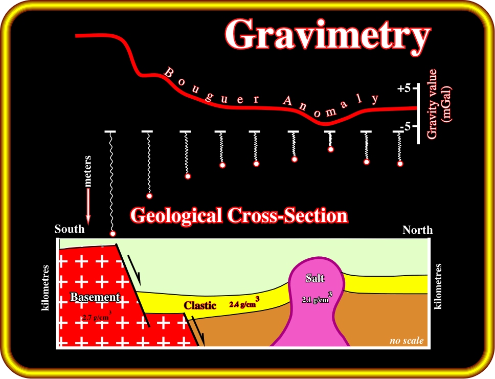
Plate 6- The relatively low density of salt with respect to its surroundings renders the salt dome a zone of anomalously low mass. Earth‘s gravitational field is perturbed by subsurface mass distributions and the salt dome therefore gives rise to a gravity anomaly that is negative with respect to surrounding areas, as illustrated on the Bouguer anomaly. As gravimetry is a deterministic method, that is to say, an a priori geological interpretation is required, which, then, can be refuted or corroborated by the gravimetric data.
Gravity and magnetic processing sequences can be summarized as follows:
a) Pre-Processing
(i) Reading/Converting Field Tapes, (ii) -Line Definition, (iii) Data Editing, (iv) Digitizing (if unrecordable or not recorded digitally), (v)- Positions, Shot-points, and Time (if acquired on a seismic operation).
b) Basic Processing
- Meter Calibration, Base Constants and Drift.
Correction for instrumental drift is based on repeated readings at a base station at recorded times throughout the day.
- Base Station Magnetic Observation and Diurnal.
The effects of diurnal variation may be removed in several ways. For magnetics (land) a method similar to gravimeter drift monitoring may be employed in which the magnetometer is read at a fixed base station periodically throughout the day.
Magnetometers do not drift and base readings are taken solely to correct for temporal variation in the measured field. Magnetic effects of external origin cause the geomagnetic field to vary on a daily basis to produce diurnal variations. Under normal conditions (quiet days), the diurnal variation is smooth and regular and has small amplitude, being at maximum in Polar Regions. Disturbing days are distinguished by far less regular diurnal variations and involve large, short-term disturbances in the geomagnetic field, with big amplitudes (magnetic storms).
- Intersection Determination.
- Misty Adjustments.
- Systematic Corrections
- Random Error Correction
- Profiling.
- Gridding and Contouring.
- General Reduction
Before the results of gravity or magnetic surveys can be interpreted, it is necessary to correct them for all variations in the Earth‘s potential fields:
- International Gravity Formula
It is a formula expressing theoretical gravity on the surface of a specified reference ellipsoid as a function of latitude.
- Earth’s Normal Magnetic Field
The International Geomagnetic Reference Field (IGRF) defines the theoretical dipolar undisturbed magnetic field related to neck at any point on the Earth's surface. In magnetic surveying, the IGRF is used to remove from magnetic data those magnetic variations attributable to this theoretical field.
- Correction Sun / Moon motion
- Eotovos Correction
In gravity measurement, on a moving platform (ship or aircraft) a correction, for centripetal acceleration caused by east-west velocity over the surface of the rotating Earth, is necessary.
- Free Air Correction
This correction corresponds to the natural decreasing of the field with elevation, i.e., the distance between observation point and the geoid.
- Bouguer and Terrain Corrections
The Bouguer correction is a correction made to gravity data for the attraction of the rock between the station and the datum elevation (commonly sea level). If the station is below the datum elevation, for the rock missing between the station and the datum, the Bouguer correction is 0.01276 ph mgal/ft, or 0.04185 ph mgal/m, where p is the specific density of the intervening rock and h is the difference in elevation between station and datum.
Terrain corrections should be applied if the actual topographic or bathymetric surface deviates significantly from the infinite Bouguer slab. For land and underwater stations, this correction is positive because both high areas above the station and low areas below it causes a lower gravity reading than would have been observed if the land were flat. For the sea stations over relatively deep water, a negative correction may be required because of the positive influence surrounding rocks above the station water depth.
Terrain correction can be made either manually or by computer by dividing the topography into compartments and summing the individual effects at each station. This requirement can add significantly to the cost of processing gravity data.
to continue press
![]()