Basic Principles in Tectonics

3- Attempt to Classify Tectonic Regimes

Contents:
3.1- Tectonic Regimes in Sedimentary Basins
3.2- Examples

3.1- Tectonic Regimes in Sedimentary Basins

As for all classifications, the classification of tectonic regimes proposed here (fig. 74) should not be applied too strictly. Similar regimes can coexist in neighbouring regions or at adjoining periods, which are hard to distinguish. Ex: folds and strike slips faults. On the other hand, the effects of salt and shale tectonics can be locally combined with an

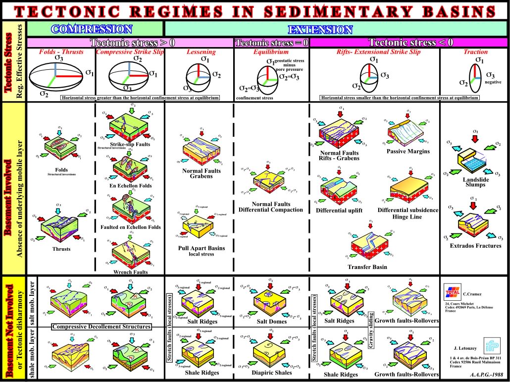
Fig.74- Classification of the tectonic regimes and associated deformations in sedimentary assuming the deformations are de consequence of a single tectonic regime.

This classification, as well as the idealized deformations in front of an orogenic belt and in a foreland platform(fig. 75) emphasizes the different regional stress ellipsoids with a lessening of the tectonic stress. They follows the philosophy of European geologists, particularly Goguel and C. A. Wegmann. However, one should not forget that:

(i) The lessening of the tectonic stress (t) is just a pedagogic hypothesis.

(ii) within a lithospheric plate, the tectonic stress is roughly constant.

(iii) The strength to deformation of the sediments that changes laterally and with depth.

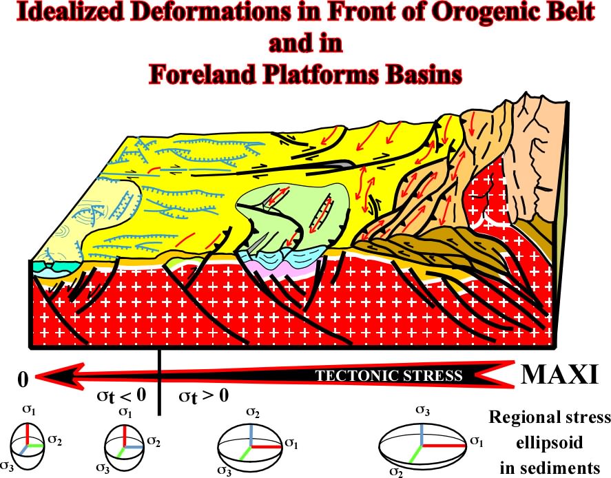
Fig. 75- Theoretically, assuming a lessening of the tectonic stress in the direction of a craton (in fact the lessing is not of the tectonic stress but the deformation threshold of the sediments), several tectonic regimes and associated deformation can be recognized between the orogenic foldbelt and the craton, that is to say, (i) thrust faults and cylindrical fold, (ii) strike-slip faults and conical folds, (iii) normal faults and associated grabens striking perpendicularly to the thrust faults of the fold belt.

To sum up, one can say that in a area affected by a unique a simple tectonic regime, the knowledge of the effective tectonic stresses allow to predict the spatial distribution of the more likely associated deformations. Such a hypothesis can be used to control the consistency, that is to say, to test the proposed structural maps and geologic cross-sections or seismic interpretations.

(i) In a first step, a geologist using the available data (maps, seismic lines cross-section) determines the more likely tectonic regime. Let’s assume that he found that the studied area was affected by a tectonic regime characterized by an ellipsoid (fig. 76) with following main axis:

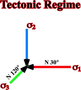
Fig.76- Firstly, this tectonic regime is characterized by a 1 horizontal striking N 30º (shortening), secondly, the 2 is vertical, that is to say that the deformation axis is mainly horizontal.

(ii) Then, taking a look at the proposed classification of the tectonic regimes illustrated in fig. 75, he easily find the more likely structures associated with such a regime, that is to say, strike-slip faults, en échellon folds, faulted en échellon folds, conical folds and wrench faults, when the basement is involved in the deformation, and compressional décollement structures when the basement is not involved (second column in the classification).

(iii) In addition, as secondary occurrence, he can find some structures of the adjacent columns, that is to say, those occurring in the “Folds-thrusts” and “Lessening” columns. All others structures shown in the classification cannot be associated with the effective “Compressive Strike Slip” tectonic regime (second column). If they exist in the studied area, they are whether anterior or posterior to the considered tectonic regime. The following examples clarify how to practically use the proposed classification.

3.2- Examples

3.2.1- Example A

This example try to illustrate how one can predict the chiefly structures in an given area using a small but significant structural map (fig. 77).

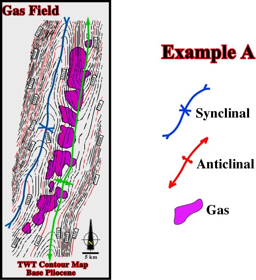
Fig. 77- This time contour map comes from a non Atlantic-type margin, that is to say, from a continental divergent margin associated with a marginal sea created by oceanization of a pre-existent back-arc basin. In other words, it can be said that the global tectonic setting of the considered area is predominantly compressional. However, one cannot forget that the occurrence of extensional tectonic regimes is necessary, since sediments cannot be shortened before being deposited. The contour map clearly indicates that folding shortened the sediments. The strike of the folds is too consistent so the interpretation is unquestionable (there are almost no chances to refute such a coherent interpretation). Therefore, as the sediments were uplifted and the structures (anticline and syncline) are cylindrical, one can say that the tectonic regime is characterized by a horizontal s1, striking more or less N 110° , a vertical 3 and a horizontal 2, striking perpendicularly to 1, that is to say, N 200°. Such a tectonic regime corresponds to the first column of the proposed classification (“Folds – Thrusts”).

The time contour map illustrated above indicates a compressional tectonic regime characterized by a horizontal 1, striking N 110°, a 3 vertical and a 2 horizontal and perpendicular to 1. The tectonic regime corresponds to the “Folds-Thrust” regime of the proposed classification (first column). Therefore, the main structures occurring in such an area (characterized by the regime) are:

- Cylindrical folds and - Thrusts.

However, as said previously, the structures on the adjacent columns, in this case those on the second column (strike-slip faults, en echelon folds, etc.), can also be found but they are subordinate. In addition, it is not relevant to know if the basement is involved or not, since the structures are akin. On the other hand, folds associated with tectonic inversions occur often in a such a tectonic regime. Actually, very often, pre-existent normal faults can be reactivated as reverse faults during this tectonic regime creating a buckling in the upper sedimentary levels. The tectonic inversions induce cylindrical folds when the angle between the s1 and the strike of the pre-existent normal fault is near 90º. When the angle is smaller the folds are conical faults.

NB- In a cylindrical fold, the s1 is perpendicular to the axial plane of the fold, that is to say, that the fold, when projected in a Wulf stereogram, falls in a meridian. In a conical fold, the s1 is oblique to the axial plane and the fold, when projected in a stereogram, falls in a paralle.

Knowing all these deductive geologic statements (considered often as a priori), geologists can easily propose interpretations difficult to refute, particularly when they adopts a criterion of relative potential satisfactoriness.

NB- This criterion characterizes as preferable interpretation that which tells us more, that is to say, the interpretation that contains the greater amount of empirical information or content, which is logically stronger, which has the greater explanatory and predictive power or which can therefore be more severely tested by comparing predicted facts with observations.

3.2.1- Example B

This example illustrates how the knowledge of the tectonic regime responsible for the deformation of the sediments, that means, the orientation of the effective stresses and the associated induced structures, can often refute well-accepted hypotheses.

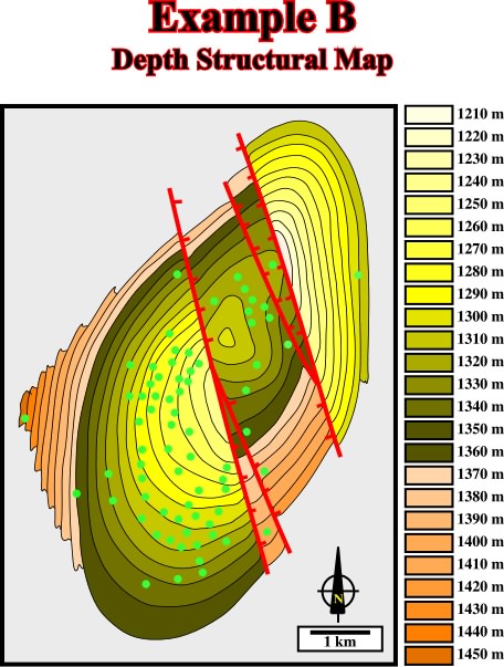
Fig. 78- This depth structural map displays the tectonic behaviour of the regional sealing interval of a large oil field located in the same area of the gas field illustrated in previous figure. So, one can say that the regional tectonic regime is characterized by a 1 horizontal striking N 130°, 2 horizontal striking N 20° and a 3 vertical. In other words, the more likely structures occurring in the area will be cylindrical folds and thrust. The structure of the seal interval looks like an anticline striking N 20-30°, with normal faults oriented N 160-170° near the apex of the structure.

The map illustrated in fig. 78, comes from the same episutural basin where the gas field (fig. 77) is located. Actually, the depicted structure belongs a basin located within the Ceno-Mesozoic megasuture, in which compressional tectonic regimes (1 horizontal) are predominant. The proposed mapping suggests that:

a) The trap of oil field is structural, that is to say, that it corresponds to a four way dips closure associated with an anticline structure.

b) The occurrence near the apex of the anticline of major normal faults, with opposite vergence.

The problem is that the normal faults are contemporaneous of the deformation. Subsequently, taking into account the regional tectonic regime (1 horizontal striking N 130°, a 2 horizontal striking N 20° and a 3 vertical) and following the proposed classification of the tectonic regimes (fig. 77), there is a strong inconsistency between the anticline structure and the normal faults in the apex of the structure.

Actually, if the faults are contemporaneous of the deformation, as it seems be the case, the structure cannot be explained by a “Folds-Thrust” tectonic regime (first column of the classification), since sediments cannot, at same time in same place, be shortened and lengthened in all directions, that is to say, that the structure cannot be an anticline. It corresponds rather to an antiform (extensional structure) induced by a shale diapir.

On the contrary, assuming that the normal faults postdate to the formation of the structure, the faults can easily be explained by an younger extensional tectonic regime (1 vertical), with the structure corresponding to an anticline structure. The hypothesis of normal faults predating the shortening is unlikely, since the faults should be reactivated as reverse, what it is not the case.

3.2.3- Example C

In this example, we will see how the knowledge of the tectonic regime can help the seismic interpreters, particularly when performing 3D interpretation, which philosophy can be summarized by the 3D block diagram of the Swiss Geologists (E. Argand, 1920, C.E. Wegmann, 1956), as illustrated in figure below (fig. 79).

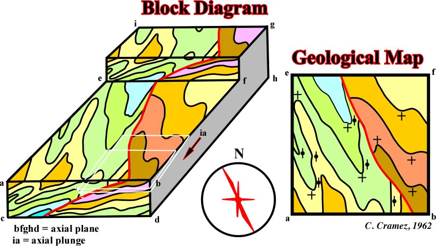
Fig. 79- This block diagram summarizes the philosophy of the 3D seismic interpretation, that is to say the interactivity between the geologic cross-sections and geologic maps (or seismic lines and seiscrops, in seismic jargon). In other words, seismic interpreters, in order to find the more likely interpretation, must interpreter not only the seismic lines, but the time slices (seiscrops) as well, which correspond to geologic maps without topography. Unfortunately, very few seismic interpreters are qualified to interpret a time slide without using the ties of the vertical seismic lines, that means that they do not use time-slices to test the profile interpretations or the profiles to test the time slice interpretation. On the contrary, they used a circular method to justify their interpretations (“verificationism”).

Let’s supposed that the seismic profile, illustrated in fig. 80, is representative of a given area. Before starting the interpretation, the seismic interpreter, which must have a strong geologic background, must, first of all, try to determine the tectonic regime responsible for the deformation of the sediments. Thus, the first important decision that he must take is to guess whether the sediments are:

a) Lengthened and b) Subsidence.

In fact, in the first hypothesis the maximum effective stress being 1 was vertical, induced:

                      (i) Lengthening;
                             (ii) Subsidence;
                                  (iii) Relative sea level rise and subsequently
                                        (iv) Deposition.

In the second hypothesis, the s1 being horizontal induced:

                     (i) Shortening;
                           (ii) Uplift;
                                 (iii) Relative sea level fall and so
                                       (iv) Erosional surface (unconformity).

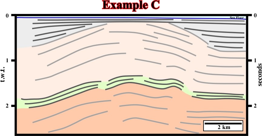
Fig. 80- This seismic profile (N-S) is representative of the area where it was shot. It is perpendicular to the structural trend. Therefore, one can say that sediments were shortened and uplifted. So, the maximum effective stress, 1, was horizontal and striking N-S. In other words, in the area, the predominant structures are (i) cylindrical folds, (ii) folds associated with tectonic inversions and (ii) thrust or reverse faults. It is relevant to point out that in a reverse fault the shortened faulted block is almost always the up-thrown block, as illustrated (reverse fault around 2 seconds, in the left part of the line). On the other hand, taking into account the different thickness of the faulted blocks (upthrown block is thicker) it is not reluctant to hypothesize the large anticline structure is associated with a tectonic inversion of a pre-existent normal fault.

Taking into account the orientation of the seismic line (fig. 80), and the its informative empiric content, one can predict that the more likely tectonic regime responsible for the deformation was characterized by a tri-axial ellipsoid of the stresses with the axes:

1 horizontal striking N-S, 2 horizontal striking W-E and 3 vertical

Knowing the tectonic regime, the interpreter should anticipate that more likely structures are:

(i) Cylindrical Folds, (ii) Folds induced by Tectonic inversion and (iii) Thrusts and Reverse faults

Strike slip-faults, en-échellon folds, faulted en-échellon folds and wrench faults are also possible, particularly as a consequence of reactivation of pre-existent structures (tectonic heritage). So, picking in a time slice (geological map without topography) the lineations (faults and structural trends), the interpreter can predict the more likely spatial location of chiefly structures whether folds or faults as shown in the geological map illustrated in fig. 81.

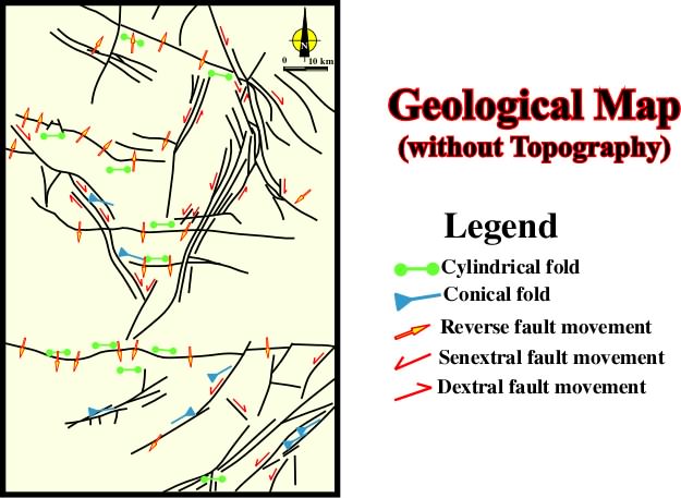
Fig. 81- On this map, the lines in black are the lineations recognized in a time slice (time geologic map without topography) in the same area of the seismic line illustrated in fig. 80. So, the interpreter knows that the tectonic regime responsible for the deformation is compressional (sediments are shortened) and characterized by a 1 horizontal striking N-S, and a 3 vertical. Consequently, he can predicted the spatial location of the more likely structures occurring in the time slice, taking into account that some of the lineations can be an inheritance from previous tectonic regimes whether compressional (1 horizontal) or extensional 1 vertical).

In a time slice, which corresponds to a geologic map with a flat topography, the easiest task of a seismic interpreter is to map the lineations (non genetic term for locally or regional linear structures). Indeed, they correspond to sharp discontinuity surfaces between different geologic or geometric realm (faults, fold axis, etc.). In fig. 81, the black lines emphasize the major lineations in a time slice of the area similar to the one where the line, illustrated in fig. 80, was shot. So, knowing that the tectonic regime in the area, suggested by the seismic line, was compressional and characterized by the following effective stresses:

1 horizontal, striking N-S; 2 horizontal, striking E-W; 3 vertical,

it is quite easy to predict, on the time slice, the more likely spatial location of the main structure (fig. 81). Potential cylindrical folds are depicted in green. Potential conical folds (associated with strike slip faults) are depicted in blue. The reverse or thrust faults, which strike perpendicular to the 1 are represented by red arrows, while the strike slip faults are indicated by the relative movement of the faulted blocks.

It is relevant here to point out that strike slip faults, with different relative movements, can strike in all directions since a lot of inherited lineations are reactivated. Geologists to determine the relative movement of the faulted blocks during reactivations use often the rosette diagram illustrated in fig. 82.

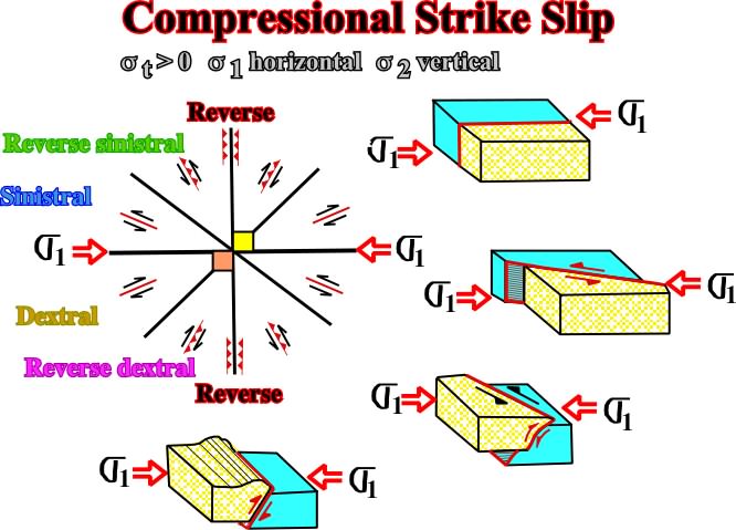
Fig. 82- Assuming lineations in all directions and a 1 striking N-S, all lineations will be reactivated. Reactivation depends on the angle between a lineation and 1. When the angle is nil, there is not reactivation. When it is 90°, the reactivation is maximum and the pre-existent fault plane is reactivated as reverse. Between these extremes, (i) reverse sinistral, (ii) sinistral, (iii) dextral and (iv) reversal dextral are possible. In such a tectonic regime only dextral and sinistral strike slip faults are neo-created. Reactivation of old pre-fractured or weak zones induce all others.

3.2.4- Example D

Very often, as illustrated on the block diagram of fig. 79, the geometry of outcrops, or superficial structures, does not often reflect the complexity of the structures at depth. Indeed, as suggested by Goguel's law (2sd Law of Thermodynamics applied to Geology), volume problems are much more important in depth than on the surface. This is easily recognized on geological cross-sections and seismic lines (fig. 83).

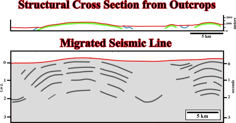
Fig. 83- On the above geological cross-section it is relatively difficult to corroborate the volume problems in depth. On the contrary, it clearly indicates the sediments were shortened and uplift. Subsequently, one can say that the tectonic regimes responsible of the shortening was charcterized by a 1 horizintal and a 3, and the more likely structures are cylindrical folds, reverse faults and thrusts. Such a knowledge, strongly help the interpreation of the seismic line (roughly parallel to the cross-section). Indeed, in depth, the sediments accommodated to the volume problems mainly by reverse faults, which are difficult to recognize on the upper levels and in surface.

The interpretation of seismic lines, as the one illustrated in fig. 83, is greatly facilitated when the interpreter knows a priori, or determines before the interpretation, the tectonic regime of the area where the line was shot. Knowing the tectonic regime of the area is compressional, with a 3 vertical, the interpreter are going to associate the marker discontinuity to reverse faults and not to normal faults (naive interpretation). In fact, as illustrate previous, normal faults cannot be associated with compressional tectoni regime. If there are normal faults on a seismic line, they are associated with extensional tectonic regime, they are either pre- or post-compression, since they cannot be developed when 1 is horizontal.

Before ending these chapter, it is relevant here to point out that certain structures as faults can be explained by different mechanism (fig. 84). Very often, in a structural interpretation, the main aim of the interpreter is to decide what is the preferable mechanism, i.e., the mechanism which contains the greater amount of empirical information, that is certainly not the more probably (in the sense of the mathematical probability).

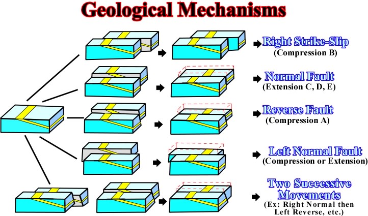
Fig. 84- Diagram illustrating that a flat geological map or in a time slice, different mechanisms can be invoked to explain observed data. The interpreter must decide what is the preferable mechanism (criterion of relative potential satisfactoriness, K. Popper, 1978).

It must be noticed that block diagrams hereabove have a flat topography, which is an ideal geological situation. The topography complicates the recognition of the movement of the faults, particularly, when they are intersected by others faults (see later).

to continue press next