Universidade Fernando Pessoa
Porto, Portugal
(ii) Bending
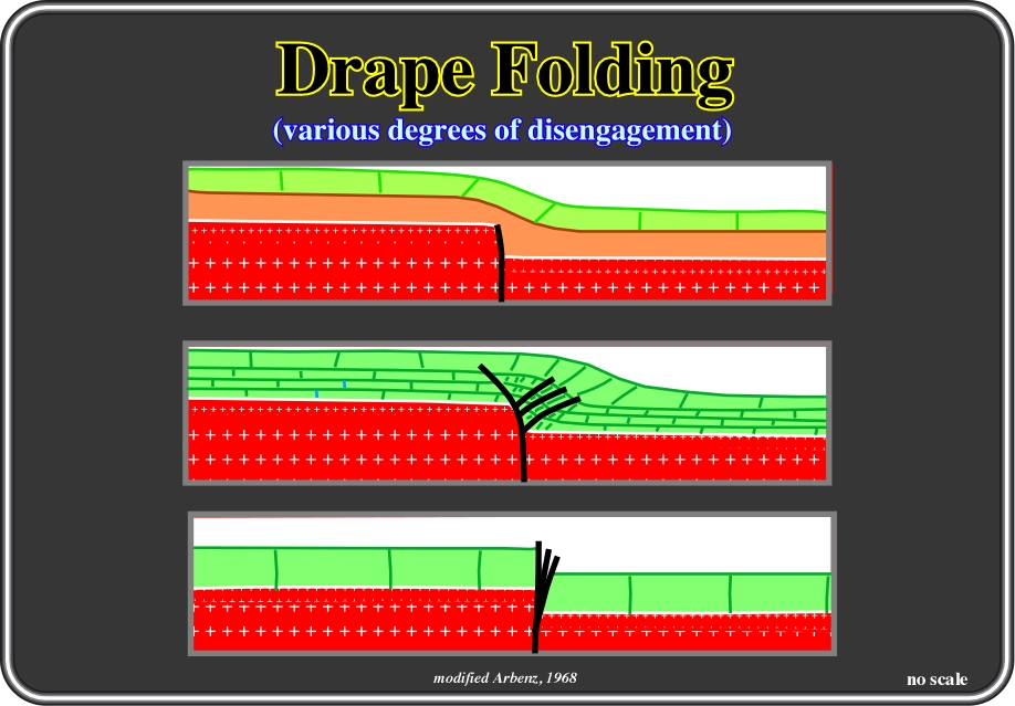
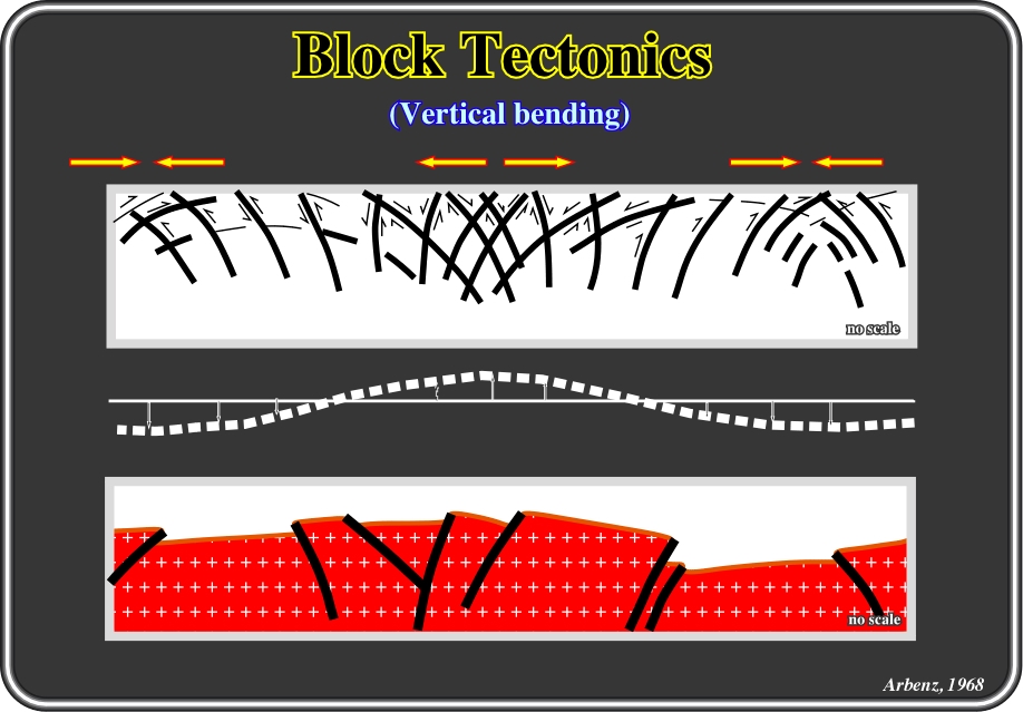
Bending is the term used to describe the flexuring of a layer induced by compression acting at high angles to layering. Geological flexures that are the result of bending are known as drape folds (Fig. 71). They are frequently formed when sediments, which cover a more rigid basement, flex in response to components of vertical movement along basement faults. This kind of tectonic style is known as block tectonics.
Drape folds are associated with block tectonic style, which is characterized by the existence of a rigid substratum within the realm of observation that has failed, in response to the primary regional stress, by faulting, producing a displaced mosaic of blocks to which the overlying strata respond passively by attempting to imitate the patterns of the rigid block mosaic either by faulting or by drape folding. The faults themselves can be normal, vertical or reverse and therefore originate from different tectonic regimes.
Fig. 71- Drape folding, as illustrate above, is true bending of one, or several, sedimentary layers in mechanical terms (as opposed to buckling) where the degree of deformation of the bent layer is proportional to the load applied to it. Drape folding over a closed spaced blockfaulted substratum does not look unlike buckle folding and the decision which of the two is present is not always easily made. One major problem of resolving drape folding is that the length of the overlying sediment layer, or layers, appears greater than the length of the original unfaulted surface of the substratum. Notice that the geometry of the fault plane is quite local. In fact, at large scale the fault plane flats in depth for the reasons said formerly.
As illustrated in Fig. 71, where three different rocks overly a crystalline basement, the lithology of the overlying rocks determines to large extent whether the fault separating two blocks in a brittle substratum continues upward into the sediment and dies out. Indeed, when block tectonics is caused by crystalline basement, then almost invariably a great contrast in ductibility exists, in spite of the fact that the presence of bedding alone introduce a strong anisotropy in the overburden.
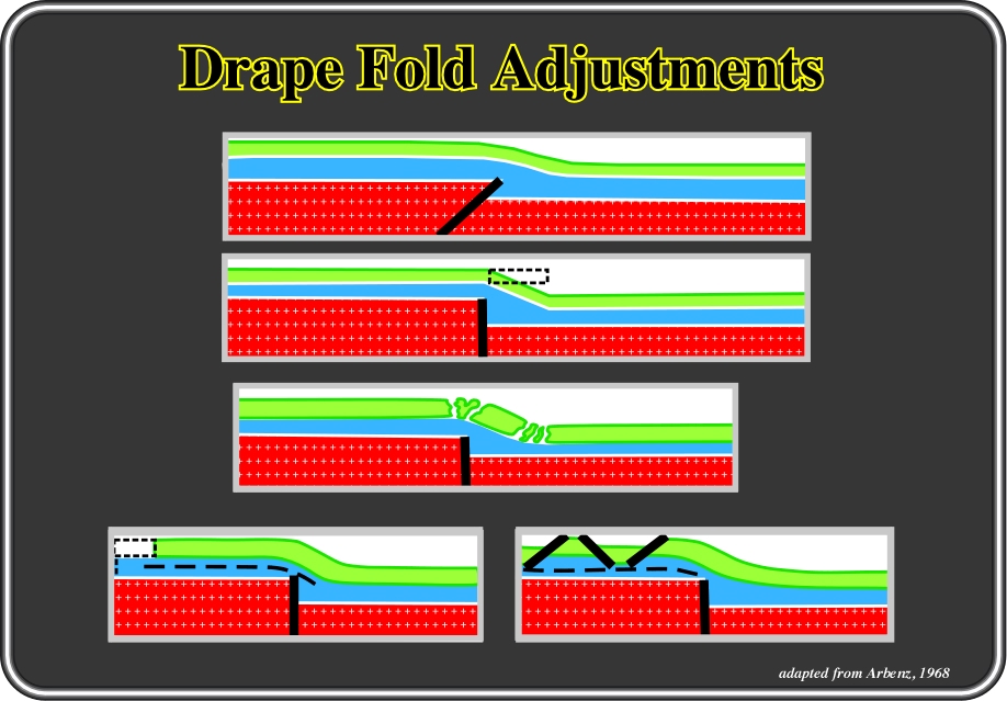
One major problem of resolving drape folding is that the length of the overlying sediment layer, or layers, appears greater than the length of the original unfaulted surface of the substratum. Several methods of readjustment of the length in drape folds are known (Fig. 72).
Fig. 72- These sketches illustrate four ways in which the length discrepancy (overlying sediments appear greater than the length of the original unfaulted surface of the substratum) can be accounted for. All of these readjustments are known to exist on ground and on seismic data, as we will see later. The closeness of resemblance of the drape fold pattern to the blockfault pattern underneath depends on the thickness of the sediments involved and on the relative ductility of the stratigraphic section (Arbenz, 1968).
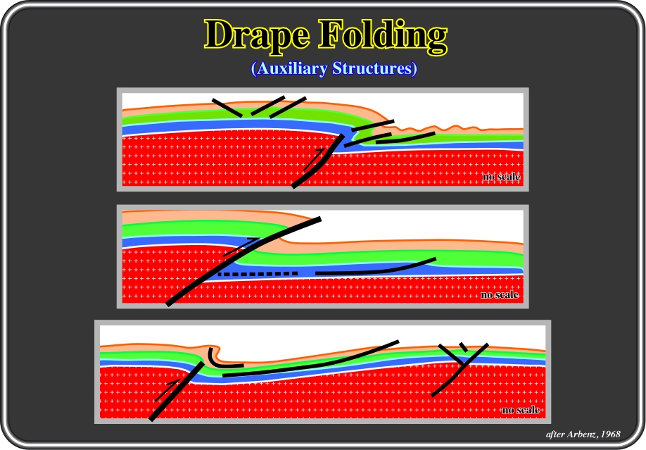
Fig. 73- The process of drape folding sets up a number of local extension and compressional tectonic regimes which may in turn deform the participing beds.
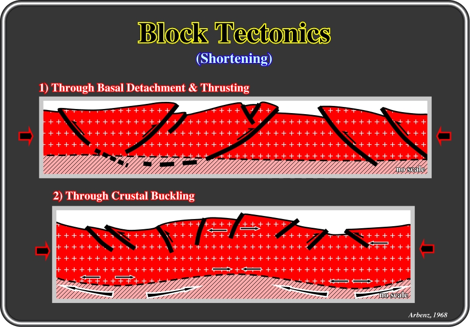
Fig.74- As said previously, block tectonics must be considered a descriptive tectonic style, describing the general character of certain geologic provinces, rather a genetic one. In fact, three main genetic styles considered: (a) compression, (b) extension and (c) vertical bending. Above the two possibilities related with a compressional regime are illustrated. In the upper sketch (1), the base of the crust undergoes a sole failure along which the thrusts flatten out and die towards depth, and in the lower (2), large scale buckling of the crust is predominant.
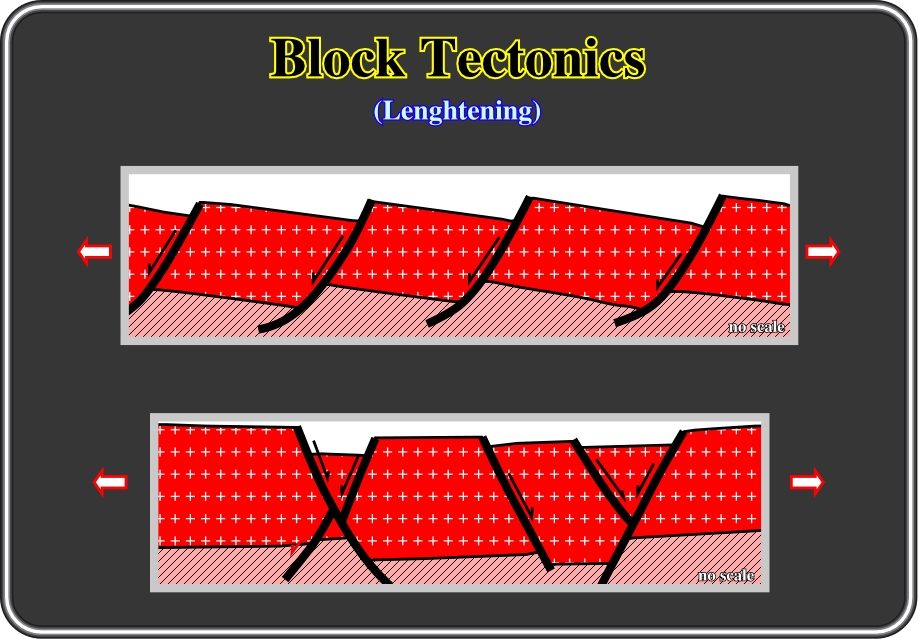
Fig. 75- Extension may become so extreme that upwelled crustal material will occupy the gaps separating the blocks of the original crust. This mechanism has been proposed for many recent rift systems in conjunction with the theory of continental drift and ocean floor separation.
Fig. 76- The third possibility case of crustal deformation leading to block tectonics is regional subcrustal or intercrustal differential vertical uplift and subsidence. This leads to similar stress distributions as one would expect under crustal buckling, namely, regions of crustal extension alternating with regions of crustal compression. The great difficulty of assigning a proper origin to a given block tectonic region is that one commonly does not know the attitude of the fault planes at depth with exception of some reverse faults where sediment can be recognized to continue underneath a basement overhang. The question of the origin in most instances, therefore, remains speculative.
The folding of layered cover rocks as the result of dip-slip movement has been termed forced folding by Strearns (1978), who argues that the overall trend and shape of such folds will be dominated by the shape of some forcing members(s) from below.
Gentle drape folds of considerable lateral extent may develop as the result of differential compaction, as when a relatively rigid block of limestone grades laterally into mudstone, which originally possessed high porosity (void spaces). Indeed, as compaction takes place, the void spaces in the mudstone close and the vertical thickness of the mudstone decreases.
Flexural slip folds form when folding occurs by:
(i) bending of the layers,
(ii) slip between the layers,
(iii) while keeping the layer thickness unchanged by folding.
Flexural slip folds are typical for low-metamorphic grades and/or rocks with a strong anisotropy (good layering). The best analog is bending a phone book, where volume preservation is accommodated by slip between the pages of the book. There are two end-member types of flexural slip folds (Fig. 77):
(A) Concentric folds, where the bending is distributed (not localised).
(B) Kink folds, where the limbs are straight and the bending is strongly localised in a sharp fold hinge.
Concentric folding normally leads to space problems in the cores of the folds (Fig. 77- c). These problems can be solved by the creation of open space, which then normally gets filled with vein material (quartz, calcite). The so-called saddle reefs can be important sites for metal deposition, particularly gold.
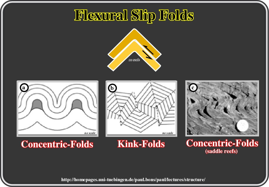
Fig. 77- In flexural slip folds, one can differentiate: (a) Concentric folds, which lead to space problems in the cores of the fold and adaptation structures, like saddle reefs must form and (b) Kink folds (often have non-parallel axial planes). In (c) is illustrated a real example of concentric folding with open saddle reefs in laminated siltstones from near Yudnamutana, South Australia.
b.7) Contractional Fault-bend Folding
Displacement along contractional faults should vary in a consistent manner, both in terms of magnitude and sense of offset. In other words, in detached contractional settings, displacement commonly occurs along reverse faults and dies up-section in the direction of transport, commonly in the cores of genetically related folds (fig. 78).
Abrupt changes in displacement magnitude and or/sense of offset should be examined carefully. Such abrupt changes may be manifested in cross sections by incompatible flat lengths between corresponding hanging-wall and footwall flats (Fig. 78), by individual layers exhibiting a sharp increase in displacement with respect to adjacent layers, or by a change in sense of offset along the fault by (i) variation in displacement magnitude and /or (ii) the fault cutting downsection in the direction of transport (Wilkerson, M.S. et Dickens, C. L., 2001).
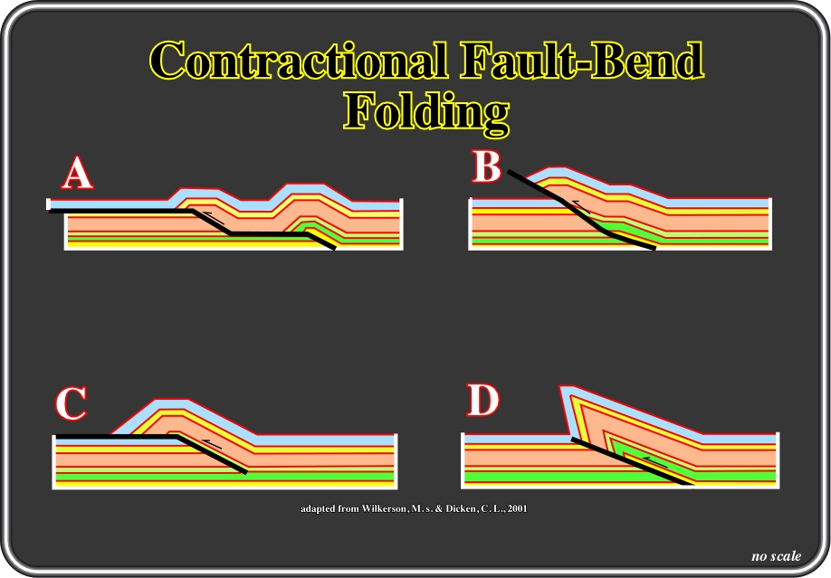
Fig. 78- In A, the hanging-wall flat is no longer than the corresponding footwall flat. In B, individual layers have experienced abrupt increases in displacement relative to adjacent layers. In C, Stratigraphic cutoffs show a reversal offset along the fault. In D, the reverse fault cuts downsection in the direction of transport.
At this point, it is interesting to review the contractional fault-bend folding model proposed by several authors (Suppe, J., 1983; Mount V. S. et al, 1990, Lacazette, 200, etc.), which constraints and assumptions were summarized by Lacaze (2000) as following:
- Bed length is conserved.
- Bed thickness is conserved.
- Flexural-slip deformation only.
Flexural-slip is simple-shear deformation (slip along bedding combined with flexure of the strata). Flexural-slip is what happens when you bend a deck of cards.
- No out of plane movement.
The model of fault-bend folding can be applied in either 2 or 3 D. 2D models assume conservation of material in the transport plane, i.e. rocks are assumed to move in a vertical plane parallel to regional transport vector.
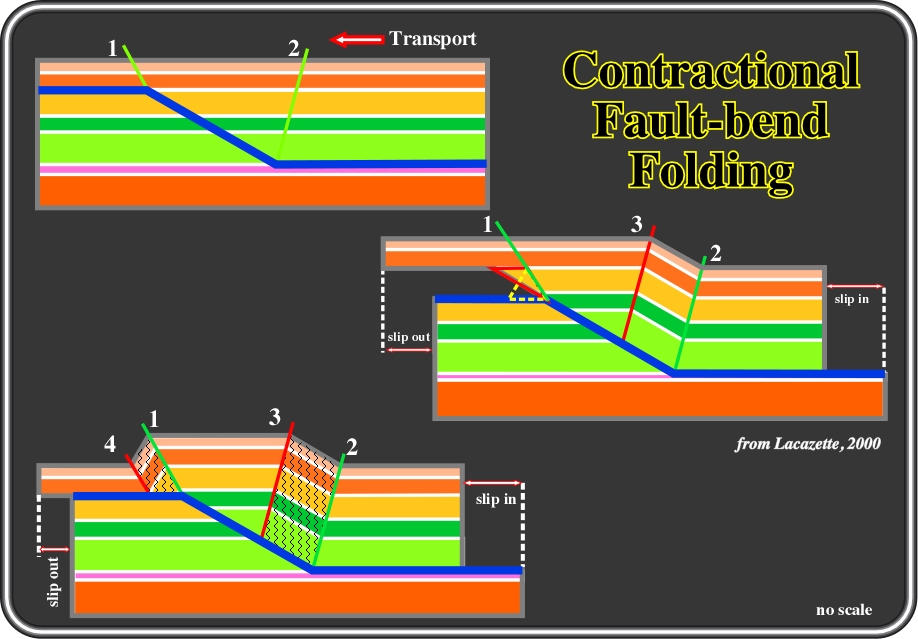
Fig. 79- Thrust faults typically run parallel to bedding in weak horizons (such as shales) and then ramp steeply through competent stratigraphic packages (such as carbonates) until they encounter another weak horizon, as illustrated above. Folding begins at the active axial planes (green) as soon as the hangingwall block begins moving. Folding at the base of the ramp is easy to visualize. As flat-lying strata are pushed onto the ramp they fold to match the ramp angle at axial plane 2. Some slip is consumed by this folding process. The folding process at the top of the ramp is less obvious. Clearly, strata above the ramp cut-off do not fold as long as they are above the ramp. At the top of the ramp the strata must collapse along axial plane 1 to fill the void. Strata within the red triangle fold to form the dashed yellow triangle, which has the same area as the red one. Substantial slip is consumed by this folding process. The stage on the bottom of the figure is known as the anticline growth stage. Active axial planes (green) do not move because they are pinned to the fault bends. Inactive axial planes (red) move with the hangingwall block. Rocks that have been folded are more likely to be fractured (gray). Most of the fault slip coming into the structure is consumed by anticline growth. Consequently, the slip-rate of the fault on the upper flat (above/in front of the ramp) is substantially lower than the slip-rate on the lower flat (below/behind the ramp). The slip-rate on the ramp above axial plane 2 is somewhat lower than the slip-rate on the lower flat. Strictly speaking, fracture development invalidates the modeling assumptions of constant bed-length and bed-thickness because fracture development allows non-recoverable rock strain. However, in many cases this strain is not significant. If slip-rate is a significant control on fault zone and fault-damage zone development, then slip-rate variations may affect fault permeability and leakage.
Folding requires shear strain of the individual strata that lie between slip surfaces as well as of the entire stratigraphic column. The type of strain required by this model is termed simple shear. When you push a deck of cards so that it slides to form a stack with slanted edges, you have deformed the deck of cards by simple shear. The type and amount of shear at each active axial plane can be calculated directly from the model. Unfortunately, this model does not accurately represent all aspects of natural folding. This model works well for analysing large structures because the entire stack of strata does appear to deform by flexural-slip in nature. However, individual strata between slip-surfaces do not deform internally by simple shear so strain predictions from this model are not a good predictor of fracture system properties.
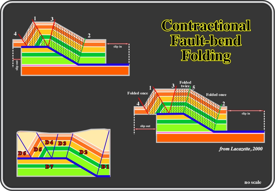
Fig. 80- The next stage is the end of anticline growth. Indeed, when the axial plane 3 has reached the top of the ramp, most of the strata that overlie the ramp have been folded, but the triangle between axial planes 1 and 3 still has not been folded. Inactive axial planes (red) move with the hangingwall block. Then, the anticline broadening stage starts. Active folding commences at the top of the ramp at axial plane 5 which forms when axial plane 3 is transported past the top of the ramp and out along the flat. Axial plane 1 becomes inactive when this happens. Folding at axial plane 5 refolds strata that were previously folded at axial plane 2. The triangular area between axial planes 1 and 3 is never folded. Rocks forward (to the left in this case) of axial plane 5 are transported passively. Slip is not consumed by folding during anticline broadening, so the slip-rate is the same along the entire fault. The implications for reservoir geology, for instance, can be summarized as follows: (i) at least seven different structure/fracture domains are present in this simple, idealized cross-section ( D1-D7 in the left bottom figure). The top of this anticline is composed of two very different structural domains even though the structure and stratigraphy appear identical in maps and cross-sections. This point is important because structural experts working in the oil industry normally do not differentiate domain D4 from D3 in maps and cross-sections because quantitative structural analysis is usually done only to define structural traps, not the flexure history of packages of rock. Fracturing of the forelimb and backlimb occurred under different conditions so that D2 and D5 may be very different geologically. In theory, D1, D4, D6 and D7 are undeformed so that on average the types and density of fractures and other minor structures should be the same in each domain. In nature, D1, D4 and D6 were transported in different relative positions so each domain may have suffered some fracturing and each domain may have somewhat different fluid-transport properties. However, given that the packages were passively transported, they should be much less fractured than the other domains. Fracturing and other reservoir-scale deformation features observed in outcrops may closely resemble reservoir rock deformation because structural domains can extend to the surface.
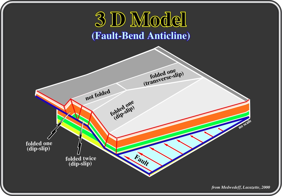
Fig. 81- This figure is a three-dimensional view of a fault-bend fold anticline, in which the plunging nose of the anticline results from decreasing displacement along the fault. Each plunging nose has an additional structural domain that was folded by transverse flexural-slip, which is slip parallel to the fold axis and perpendicular to the transport direction. Development of the plunging fold nose requires transverse extension of the folded rocks, which violates the constant bed-length constraint used in 2-D models. This extension is accommodated by fractures. In theory, transverse flexural-slip can distribute the strain across the entire fold. In nature, fractures are often concentrated in the plunging fold noses where the transverse extension is concentrated. The amount of fold-axis parallel extension as estimated from quantitative structural analysis of seismic data provides a direct estimate of the fracture strain, but not of the fracture porosity. The flat-lying rocks ahead of and behind the fold (Domains D1 and D6 in Figure 6) have also been transversely extended due to the change in displacement along the fault and should be fractured. Plunging fold noses also can form at lateral ramps, which are fault ramps that strike parallel to the transport direction. Regardless of the mechanism that causes fold closure, the strata in any plunging fold must have been extended transversely.
In their "Easy guide to Kinks" Web page (http://www.eas.purdue.edu/physproc/HTM%2520Files/easy%5Fguide%Fto%5Fkinks.htm) Johnson, K. M. and Jeffrey D. Manuszak, consider that a kink band is the fundamental building block of kink folds, that is to say, a tabular shear zone that cuts across layered media such as bedding, foliation, crystal lattices or cleavage planes and that is characterized by a monocline with an inner limb, in which the layering has been reoriented with respect to that in the two outer limbs (Fig. 82).
There are three variants of kink folds (fig. 82):
(i) Symmetric conjugate,
(ii) Asymmetric conjugate, and
(iii) Monoclinal kink folds.
The symmetric conjugate kink fold (fig. 82-A) indicates negligible layer-parallel shear stress. The asymmetric conjugate kink fold shown in fig. 82-B indicates significant left-lateral, layer-parallel shear stress. The monoclinal kink fold shown in fig. 82-C indicates greater left-lateral layer-parallel shear stress. If the layer-parallel shear stress is reversed, the asymmetries of the fold forms are reversed. We see in fig. 82-B that the asymmetric conjugate kink fold has the same sense of asymmetry as the drag fold in fig. 82-D. In both cases, right-lateral shearing is applied and the short limb is facing right. The facing direction of the steeper limb is reversed if the sense of shear is reversed. The monoclinal kink fold, however, has the opposite sense of asymmetry (fig. 82-C) from drag folds and asymmetric, conjugate kink folds. Thus the problem is that one cannot apply the intuitive notion to some kinds of kink folds that the facing direction of the steeper limb of an asymmetric fold indicates the direction of layer-parallel shear.
The central problem of interpreting the sense of shear of asymmetric folds is therefore the determination of the kind of fold one is studying. One must be able to recognize three kinds of asymmetric folds-drag (or parasitic) folds (fig. 82-D), asymmetric, conjugate kink folds (fig. 82-B) and monoclinal kink folds (fig. 82-C).
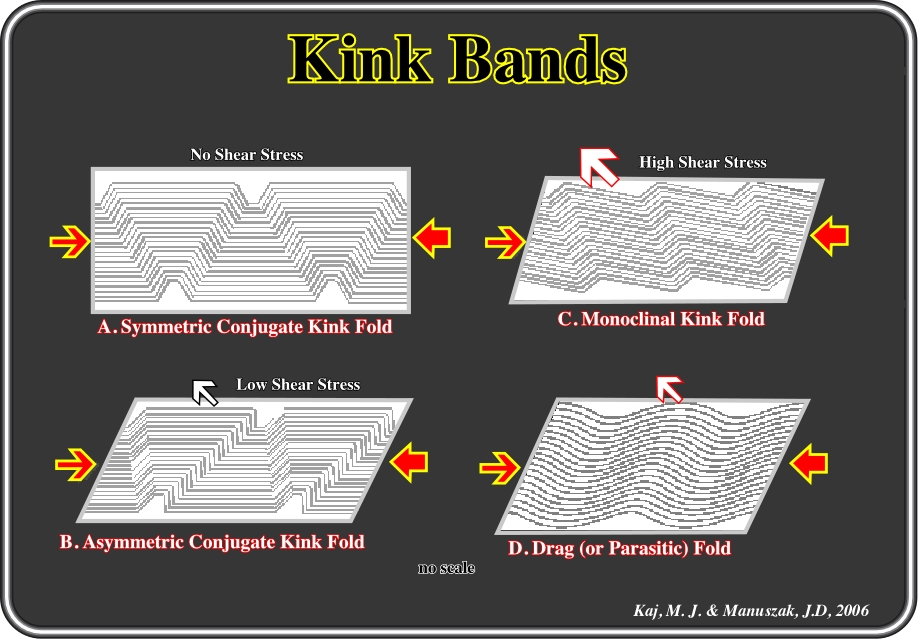
Fig. 82- In this figure, kink and drag folds formed under layer-parallel compression are illustrated. In A, symmetric conjugate kink folds, produced by layer-parallel compression (zero layer-parallel shear), contain identical kink bands facing left and right. In B, asymmetric conjugate kink folds, which are created by right-lateral layer-parallel shear stress are illustrated. In C, asymmetric monoclinal kink folds, in which larger right-lateral shear causes only left-facing limbs to form are shown. In D, drag (or parasitic) fold with the shorter limb facing rightward is drawn.
Kink bands occur in strongly anisotropic rock where the anisotropy is either beds with a finite thickness or foliation with very thin layers. These two are fundamentally different types of geological material that kink in different manners.
- The first is well cleaved schist where individual microlithons are very thin. This material resembles a pack of computer cards where folding is vary sharp at the hinges.
- In the second geological material the bedding has a finite thickness where any folding at the hinges has to respond to the thickness of the hinges. Kinks in bedded material resemble the common chevron folds.
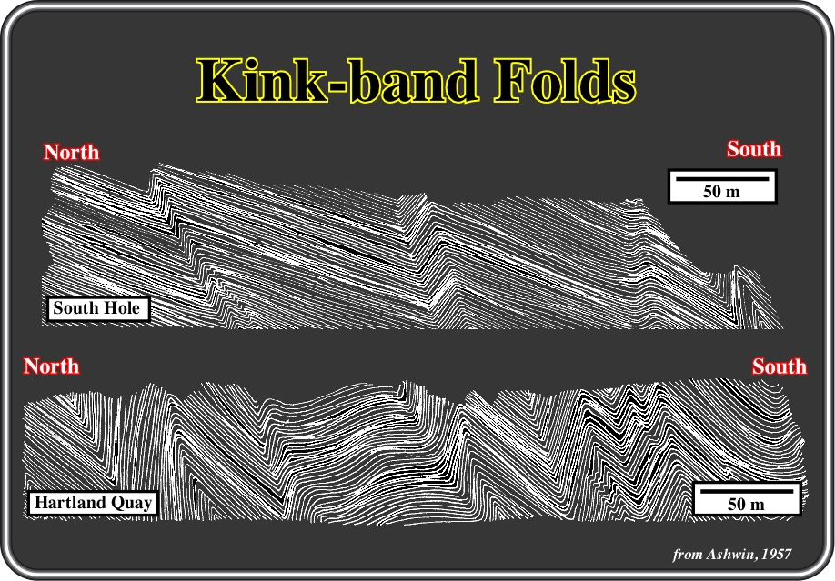
Fig. 83- Kink-band folds developed in turbidite sediments in a cliff section at N. Devon, England.
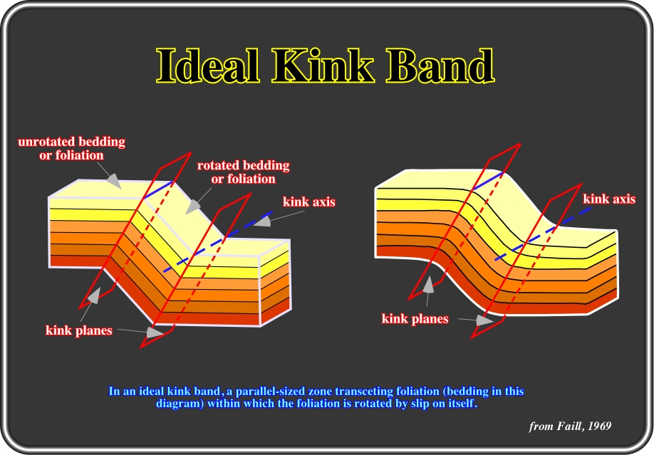
Fig. 84- Kink bands are geometrically related to chevron folds and are probably formed in a similar manner. The internal deformation within kink zones is generally accomplished by flexural slip on the layering. The layers are bent at the hinge and the orthogonal thickness of the layers is generally nearly constant throughout the fold. The axial surface of each fold usually lies close to the bisector of the angle between the straight limbs. Occasionally, the axis surface makes a smaller angle with the dominant trend of the layering than it does with the layering in the kink zones.

Fig. 85- This sketches illustrate the chief difference between a fold (buckling) formed above a décollement surface and a kink-band fold. The intersection of the external opposite kink-planes gives the top of mobile layers. Often, volume problems occur at the base of the kink-bands (see fig. 86).
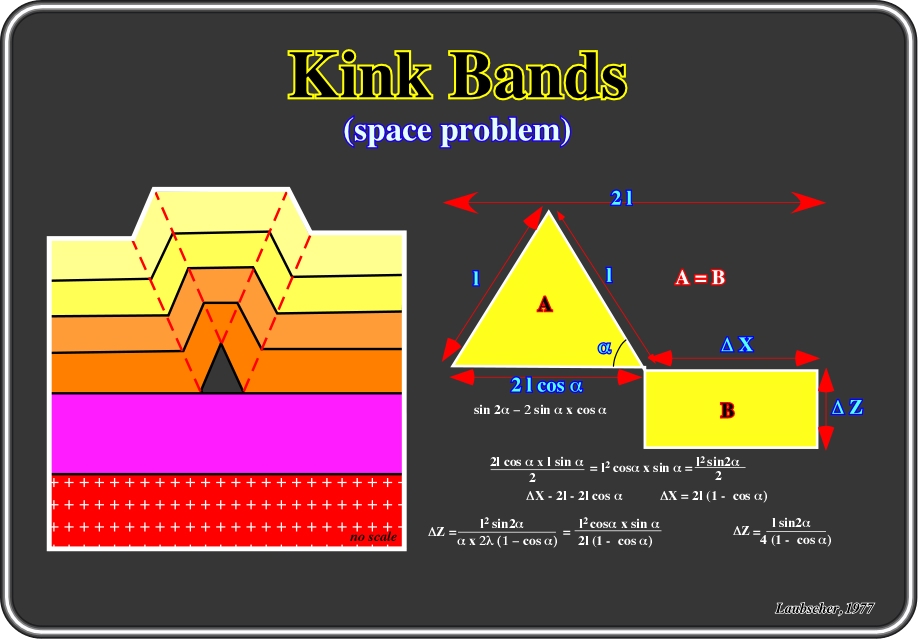
Fig. 86- Kink-bands create a space problem immediately above the detachment surface. For an estimate of the importance of the underlying mobile layer thickness it may be assumed (very schematically) that its compression is achieved by means of the elimination masses used to fill the basal triangular space of the kink bands. For an quick calculation the
z = f (a,l), Laubscher’s method is often used.
The kink method can be used to pick fault planes, on seismic lines (Fig. 87) or to restore geological sections (Fig. 88) in order to test volume preservation, i.e. the consistence of the interpretations. This method can only be used in compressional tectonic regimes since it supposes a bed to bed movement, which, generally, it is not observed in extensional tectonic regimes. The method can be presented in several basic steps:
A) Location of areas of homogeneous dip.
B) Location of axial surfaces between areas of homogeneous dip.
C) Location of major discontinuities where the axial surfaces terminate or branch.
D) Interpretation of terminations of axial surfaces in terms of fault trajectories.
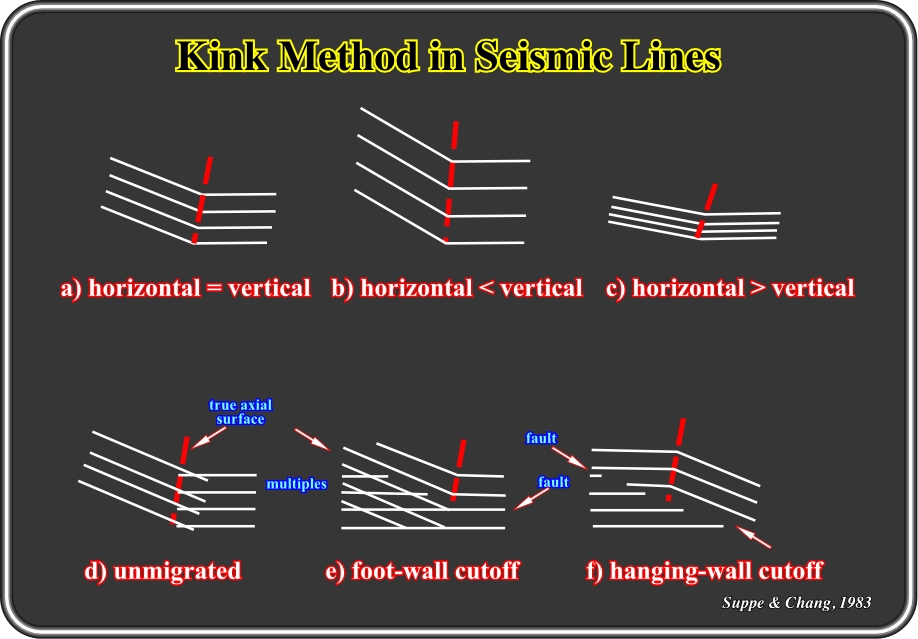
Fig. 87- These sketches illustrated the chief patterns of seismic reflectors that display kink folds. As said previously, the kink method allows the axial surfaces to be localized and fault planes to be identified on seismic lines and particularly in old unmigrated 2D seismic data.
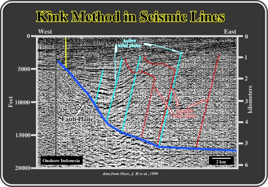
Fig. 88- here is an example of a seismic line from the onshore Sumatra, in which the interpreter used the kink method to pick the axial planes (active and inactive, see later).
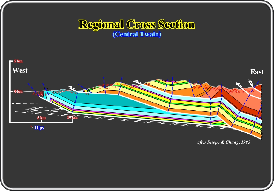
Fig. 89-This figure taken from Suppe & Chang (1983) illustrates a geological cross-section restored by kink method using the sedimentary dips measured along the ground profile. As said previously the method consists in main four steps (i) Location of areas of homogeneous dip, (ii) Location of axial surfaces between areas of homogeneous dip;, (iii) Location of major discontinuities where the axial surfaces terminate or branch, (iv) Interpretation of terminations of axial surfaces in terms of fault trajectories.
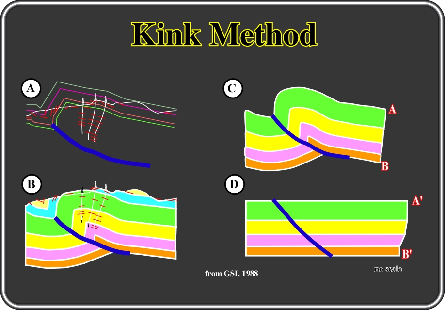
Fig. 90- In certain fold-belts, due to a karstic topography, it is almost impossible to shoot seismic lines to detect the best hydrocarbon traps. Exploration is mainly based in surface geology and drilling. So, the interpretations of dipmeter logs become an important exploration step. They allow the prediction of tectonic behaviour (A), in depth and the location of the more likely successful trap (B). Restored depth sections can then be tested in order to refute volume preservation as illustrated in C and D. (see next).
It's fairly common for folds to exhibit uniform dips for a wide interval and then change dip abruptly. The fold exhibits a series of kinks rather than smooth curvature. We can approximate such folds using the kink method. It is a bit more common these days for folds to be represented this way than with the Busk or arc method, that is to say:
- Find concentric circles tangent to two dip measurements.
- Radii of circles are always perpendicular to the tangent where the radius hits the circle.
- C onstruct perpendiculars to each dip, and the intersection of the two perpendiculars is the center of the desired arcs).
The basic method is to allow each dip measurement to define a zone where the dip is constant. The boundaries of the dip zones are the lines that bisect angles between adjacent dips. The example below begins with three different ways to find the bisector. The actual point here the fold kinks may not coincide exactly with the bisector. Why should it? If you have two dips at points 1 and 2, the change in dip could come anywhere between them, and is not necessarily going to coincide with a line halfway between the two dips. This method, like all fold construction techniques, is an approximation.
The kink method works as depicts below:
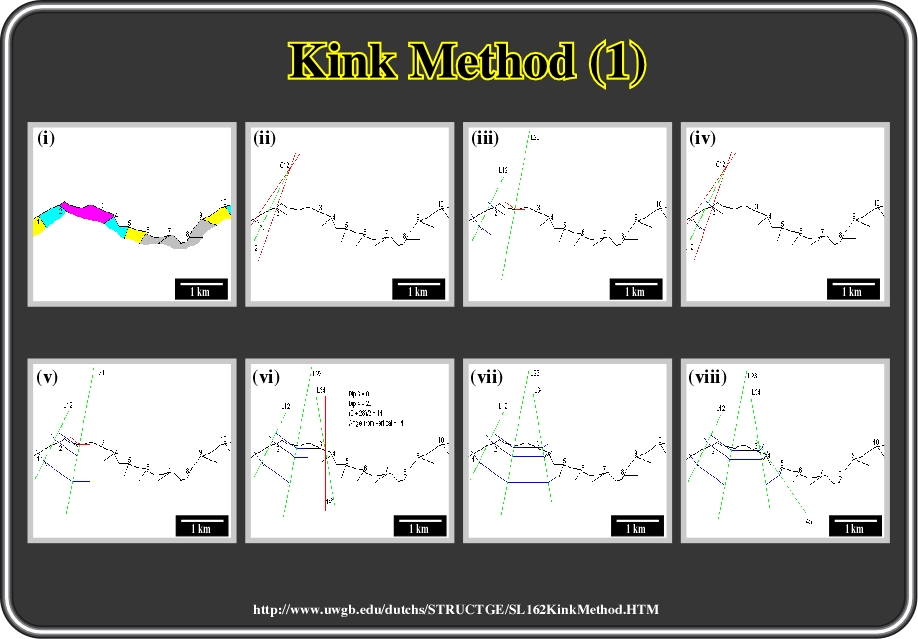
Fig. 91- (i) In the example at upper left, dip data are shown. We want to construct a cross-section that satisfies the data. The stratigraphic units are coloured here but will not be coloured for most of the remaining diagrams. It is often better not to consider stratigraphy until after the cross-section is drawn. (ii) We first find the center for concentric circles tangent to dips 1 and 2. All the circles tangent to dip 1 have their centers on a line perpendicular to dip 1. All the circles tangent to dip 2 have their centers on a line perpendicular to dip 2. Therefore, the intersection C12 is the center of concentric circles tangent both to dip 1 and to dip 2. (iii) Using C12 as a center, draw arcs tangent to dips 1 and 2 as shown. Draw the arcs only between the two perpendiculars. (iv) Now locate center C23, the center of concentric circles tangent to dips 2 and 3. You already have a line perpendicular to dip 2, so you only need to draw a line perpendicular to dip 3.Note that, as often happens, the center is off the diagram. Draw the arcs tangent to dips 2 and 3. Again, draw them only between the two perpendiculars. (v) We can now exchange information with sector 1-2. Extend the arc from dip 1 into sector 2-3, using C23 as a center (lower red arc).Extend the arc from dip 3 into sector 1-2, using C12 as a center (upper red arc). In general, as we complete the cross-section, we will extend data from one sector to the next like this. (vi) We can now construct center C34 by drawing a perpendicular to dip 4. We already have the perpendicular to dip 3.We extend the arcs from sector 2-3 into sector 3-4 as shown.Note that the arc that starts at dip 2 passes very close to dip 4. We don't need an arc through every dip, even though we may use that dip to construct a center of curvature. So we won't bother drawing an arc for dip 4. (vii) Construct center C45 by drawing a perpendicular to dip 5. We already have the perpendicular to dip 4. Extend the arcs from sector 3-4 into sector 4-5 as shown. Note that the arc that starts at dip 1 passes very close to dip 5. Again, we need not bother drawing an arc for dip 4. (viii) Construct center C56 by drawing a perpendicular to dip 6. We already have the perpendicular to dip 5. Note that the intersection is now beneath the surface. This is no problem. It means the fold is now concave downward (an anticline).
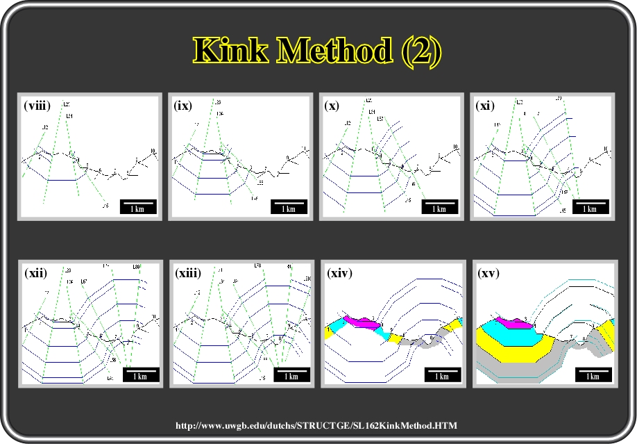
Fig. 92- (viii) construct center C56 by drawing a perpendicular to dip 6. We already have the perpendicular to dip 5. Note that the intersection is now beneath the surface. This is no problem. It means the fold is now concave downward (an anticline), (ix) Construct the arc tangent to dip 6 as shown. Since this point is stratigraphically lower than all the other datum points, we continue the arc back through all the other sectors as well (shown in red), (x) Construct arcs to connect with all the previously-constructed arcs as shown in red. (xi) Sector 6-7 completed, (xii) Sector 7-8 completed, (xiii) Sector 8-9 completed. Since point 9 falls between two already drawn arcs, there is no real need to construct another arc for it, at least for now. Note that centers C67, C78 and C89 are all close together. This simply means the fold has fairly uniform curvature over that interval. (xiv) Sector 9-10 completed. Since point 10 falls very close to an already drawn arc, there is no real need to construct another arc for it. (xv) It is virtually certain when you draw a cross section using strictly geometric methods that the contacts will not match exactly with their predicted positions. There are many reasons why not: The units will not be uniform in thickness There are small construction errors Dips are not uniform from place to place Dip measurements have small errors Folds do not have ideal geometrical shapes. Here we have indicated the stratigraphy. It is virtually certain when you draw a cross section using strictly geometric methods that the contacts will not match exactly with their predicted positions.What we need to do now is redraw the folds so the cross-section matches both the dips and the stratigraphy. (xvi) Here all the construction has been removed and the arcs are subdued. Most of the time you can modify the fold shapes by hand to match the stratigraphy without too much trouble. Modified contacts are in black.
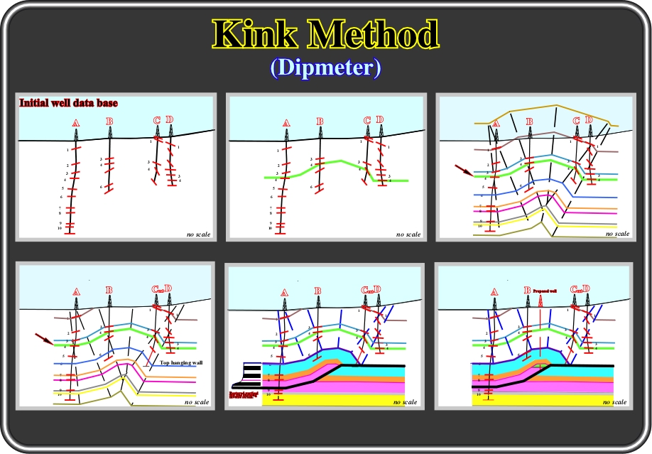
Fig. 93- The kink method using the dipmeter results can be summarized as follows: (i) using dip projection and stratigraphic correlations, a chronostratigraphic horizon (green marker) is constructed through the top of 4 formations taking into account all dip information. The geometry is projected above and below the constructed 4 top horizon (green) to check data compatibility. The well C is extended until the top of the hanging wall (downthrown block) is located. Now, the section can be quickly modified by (i) projecting the detachment plane and leading thrust fault surface abd (ii) 2) constructing the horse and its internal geometry. The horse is restored to examine the state of strain in the sheet. Complete new model with predicted horse. New strategy: Drill through top of predicted anticline to top of oil trap.
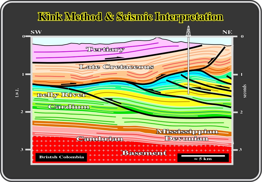
Fig. 94- Seismic line interpreted using kink method based in the chronostratigraphic reflectors and dipmeters results. In so complex areas, seismic interpretation is performed by trial and errors. Each proposed interpretation is seldom corroborated always by new data. On the contrary, it is very often refuted, which oblige geologists to advance a new interpretation, which will be more difficult to refute, i. e. more coherent (lesser falsifiable).
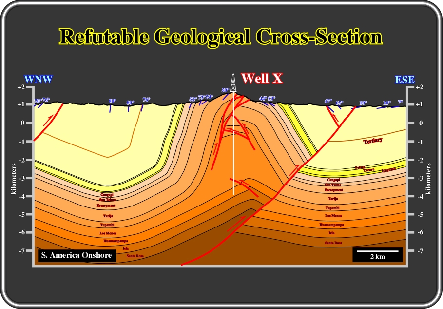
Fig. 95- As said previously, this cross-section does not respect volume preservation. In the next figures, regional cross-sections of the same area are tentative solutions to explain the sedimentary shortening and the successive steps of deformation.
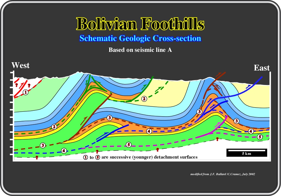
Fig. 96- Five detachment surfaces and associated anticline structures shortened the sediments. The oldest detachment (in this area) is surface 1 and the youngest is 5. They are successively deformed by the younger structures. The vertical scale was omitted for confidentiality reasons.
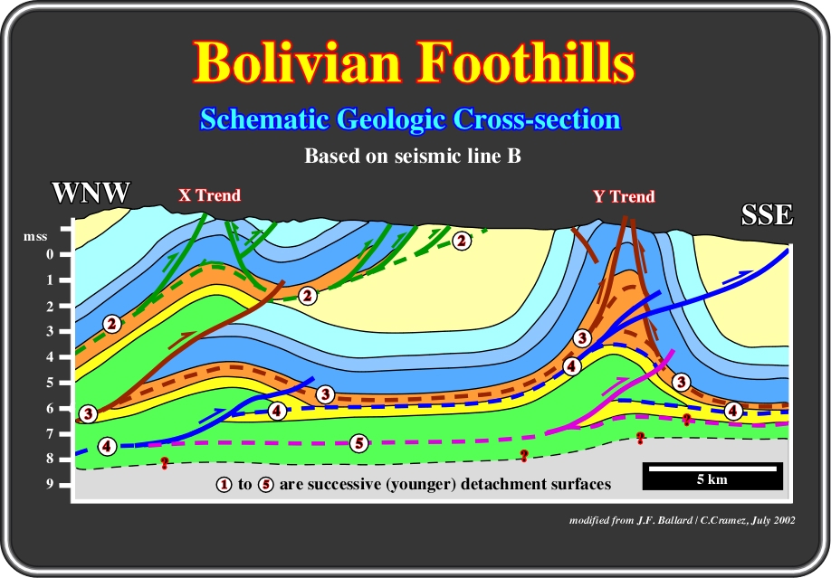
Fig. 97- The Y trend structure is here illustrated as a consequence of a multiphasic deformation, which is lesser refutable than the one proposed in fig. 2.42.
![]()
Send E-mail to ccramez@compuserve.com or cramez@ufp.pt with questions or comments about this short-course.
Copyright © 2000 CCramez
Last modification:
Agosto 27, 2006